8Theoretical BiophysicsComputational Biophysical Tools and Methods that Require a Pencil and Paper
It is nice to know that the computer understands the problem. But I would like to understand it too.
—Nobel laureate Eugene Wigner (1902–1995), one of the founders of modern quantum mechanics
General Idea: The increase in computational power and efficiency has transformed biophysics in permitting many biological questions to be tackled largely inside multicore computers. In this chapter, we discuss the development and application of several such in silico techniques, many of which benefit from computing that can be spatially delocalized both in terms of the servers running the algorithms and those manipulating and archiving significant amounts of data. However, there are also many challenging biological questions that can be tackled with theoretical biophysical tools consisting of a pencil and a piece of paper.
8.1 Introduction
Previously in this book we have discussed a range of valuable biophysical tools and techniques that can be used primarily in experimental investigations. However, biological insight from any experiment demands not only the right hardware but also a range of appropriate techniques that can, rather broadly, be described as theoretical biophysics. Ultimately, genuine insight into the operation of complex processes in biology is only gleaned by constructing a theoretical model of some sort. But this is a subtle point on which some life and physical scientists differ in their interpretation. To some biologists, a “model” is synonymous with speculation toward explaining experimental observations, embodied in a hypothesis. However, to many physical scientists, a “model” is a real structure built from sound physical and mathematical principles that can be tested robustly against the experimental data obtained, in our case from the vast armory of biophysical experimental techniques described in Chapters 3 through 7 in particular.
Theoretical biophysics methods are either directly coupled to the experiments through analyzing the results of specific experimental investigations or can be used to generate falsifiable predictions or simulate the physical processes of a particular biological system. This predictive capability is absolutely key to establishing a valuable theoretical biophysics framework, which is one that in essence contains more summed information than was used in its own construction, in other words, a model that goes beyond simply redefining/renaming physical parameters, but instead tells us something useful.
The challenges with theoretical biophysics techniques are coupled with the length and time scales of the biological processes under investigation. In this chapter, we consider regimes that extend from femtosecond fluctuations at the level of atomistic effects, up to the time scales of several seconds at the length scale of rigid body models of whole organisms. Theoretical biophysics approaches can be extended much further than this, into smaller and larger length and time scales to those described earlier, and these are discussed in Chapter 9.
We can broadly divide theoretical biophysics into continuum level analysis and discrete level approaches. Continuum approaches are largely those of pencil and paper (or pen, or quill) that enable exact mathematical solutions to be derived often involving complex differential and integral calculus approaches and include analysis of systems using, for example, reaction–diffusion kinetics, biopolymer physics modeling, fluid dynamics methods, and also classical mechanics. Discrete approaches carve up the dimensions of space and time into incrementally small chunks, for example, to probe small increments in time to explore how a system evolves stochastically and/or to divide a complex structure up into small length scale units to make them tractable in terms of mathematical analysis. Following calculations performed on these incremental units of space or time, then each can be linked together using advanced in silico (i.e., computational) tools. Nontrivial challenges lie at the interface between continuum and discrete modeling, namely, how to link the two regimes. A related issue is how to model low copy number systems using continuum approaches, for example, at some threshold concentration level, there may simply not be any biomolecule in a given region of space in a cell at a given time.
The in silico tools include a valuable range of simulation techniques spanning length and time scales from atomistic simulations through to molecular dynamics simulations (MDS). Varying degrees of coarse-graining enable larger time and length scales to be explored. Computational discretization can also be applied to biomechanical systems, for example, to use finite element analysis (FEA). A significant number of computational techniques have also been developed for image analysis.
8.2 Molecular Simulation Methods
Theoretical biophysics tools that generate positional data of molecules in a biological system are broadly divided into molecular statics (MS) and molecular dynamics (MD) simulation methods. MS algorithms utilize energy minimization of the potential energy associated with forces of attraction and repulsion on each molecule in the system and estimate its local minimum to find the zero force equilibrium positions (note that the molecular simulation community use the phrase force field in reference to a specific type of potential energy function). MS simulations have applications in nonbiological analysis of nanomaterials; however, since they convey only static equilibrium positions of molecules, they offer no obvious advantage to high-precision structural biology tools and are likely to be less valuable due to approximations made to the actual potential energy experienced by each molecule. Also, this static equilibrium view of structure can be misleading since, in practice, there is variability around an average state due to thermal fluctuations in the constituent atoms as well as surrounding water solvent molecules, in addition to quantum effects such as tunneling-mediated fluctuations around the zero-point energy state. For example, local molecular fluctuations of single atoms and side groups occur over length scales <0.5 nm over a wide time scale of ~10−15 to 0.1 s. Longer length scale rigid-body motions of up to ~1 nm for structural domains/motifs in a molecule occur over ~1 ns up to ~1 s, and larger scales motions >1 nm, such as protein unfolding events binding/unbinding of ligands to receptors, occur over time scales of ~100 ns up to thousands of seconds.
Measuring the evolution of molecular positions with time, as occurs in MD, is valuable in terms of generating biological insight. MD has a wide range of biophysical applications including simulating the folding and unfolding of certain biomolecules and their general stability, especially of proteins, the operation of ion channels, in the dynamics of phospholipid membranes, and the binding of molecules to recognition sites (e.g., ligand molecules binding to receptor complexes), in the intermediate steps involved in enzyme-catalyzed reactions, and in drug design for rationalizing the design of new pharmacological compounds (a form of in silico drug design; see Chapter 9). MD is still a relatively young discipline in biophysics, with the first publication of an MD-simulated biological process being only as far back as 1975. That was on the folding of a protein called “pancreatic trypsin inhibitor” known to inhibit an enzyme called trypsin (Levitt and Warshel, 1975).
New molecular simulation tools have also been adapted to addressing biological questions from nonbiological roots. For example, the Ising model of quantum statistical mechanics was developed to account for emergent properties of ferromagnetism. Here it can also be used to explain several emergent biological properties, such as modeling phase transition behaviors.
Powerful as they are, however, computer simulations of molecular behavior are only as good as the fundamental data and the models that go into them. It often pays to take a step back from the simulation results of all the different tools developed to really see if simulation predictions make intuitive sense or not. In fact, a core feature to molecular simulations is the ultimate need for “validation” by experimental tools. That is, when novel emergent behaviors are predicted from simulation, then it is often prudent to view them with a slightly cynical eye until experiments have really supported these theoretical findings.
8.2.1 General Principles of MD
A significant point to note concerning the structure of biomolecules determined using conventional structural biology tools (see Chapter 5), including not just proteins but also sugars and nucleic acids, is that biomolecules in a live cell in general have a highly dynamic structure, which is not adequately rendered in the pages of a typical biochemistry textbook. Ensemble-average structural determination methods of NMR, x-ray crystallography, and EM all produce experimental outputs that are biased toward the least dynamic structures. These investigations are also often performed using high local concentrations of the biomolecule in question far in excess to those found in the live cell that may result in tightly packed conformations (such as crystals) that do not exist naturally. However, the largest mean average signal measured is related to the most stable state that may not necessarily be the most probabilistic state in the functioning cell. Also, thermal fluctuations of the biomolecules due to the bombardment by surrounding water solvent molecules may result in considerable variability around a mean-average structure. Similarly, different dissolved ions can result in important differences in structural conformations that are often not recorded using standard structural biology tools.
MD can model the effects of attractive and repulsive forces due to ions and water molecules and of thermal fluctuations. The essence of MD is to theoretically determine the force F experienced by each molecule in the system being simulated in very small time intervals, typically around 1 fs (i.e., 10−15 s), starting from a predetermined set of atomic obtained from atomistic level structural biology of usually either x-ray diffraction, NMR (see Chapter 5), or sometimes homology modeling (discussed later in this chapter). Often, these starting structures can be further optimized initially using the energy minimization methods of MS simulations. After setting appropriate boundary conditions of system temperature and pressure, and the presence of any walls and external forces, the initial velocities of all atoms in the system are set. If the ith atom from a total of n has a velocity of magnitude Vi and mass mi, then, at a system temperature T, the equipartition theorem (see Chapter 2) indicates, in the very simplest ideal gas approximation of noninteracting atoms, that
(8.1)The variation of individual atomic speeds in this crude ideal gas model is characterized by the Maxwell–Boltzmann distribution, such that the probability p(vx,i) of atom i having a speed vx parallel to the x-axis is given by
(8.2)In other words, this probability distribution is a Gaussian curve with zero mean and variance
This is then used to subtract away a momentum offset from each initial atomic velocity so that the net starting momentum of the whole system is zero (to minimize computational errors due to large absolute velocity values evolving), so again for the x component
(8.4)and similarly, for y and z components. A similar correction is usually applied to set the net angular momentum to zero to prevent the simulated biomolecule from rotating, unless boundary conditions (e.g., in the case of explicit solvation, see in the following text) make this difficult to achieve in practice.
Then Newton’s second law (F = ma) is used to determine the acceleration a and ultimately the velocity v of each atom, and thus where each will be, position vector of magnitude r, after a given time (Figure 8.1), and to repeat this over a total simulation time that can be anything from ~10 ps up to several hundred nanoseconds, usually imposed by a computational limit in the absence of any coarse-graining to the simulations, in other words, to generate deterministic trajectories of atomic positions as a function of time. This method involves numerical integration over time, usually utilizing a basic algorithm called the “Verlet algorithm,” which results in low round-off errors. The Verlet algorithm is developed from a Taylor expansion of each atomic position:
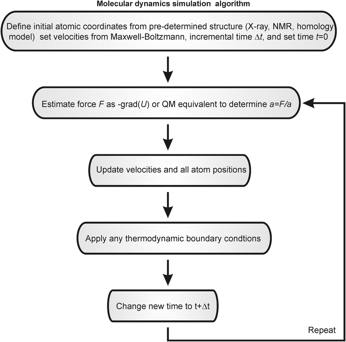
Figure 8.1 Molecular dynamics simulations (MDS). Simplified schematic of the general algorithm for performing MDS.
Thus, the error is atomic position scales as ~O((Δt)4), which is small for the femtosecond time increments normally employed, with the equivalent recursive relation for velocities having errors that scale as ~O((Δt)2). The velocity form of the Verlet algorithm most commonly used in MD can be summarized as
(8.6)Related, though less popular, variants of this Verlet numerical integration include the LeapFrog algorithm (equivalent to the Verlet integration but interpolates for velocities at half time step intervals, but has a disadvantage in that velocities are not known at the same time as the atomic positions, hence the name) and Beeman algorithm (generates identical estimates for atomic positions as the Verlet method, but uses a slightly more accurate but computationally more costly method to estimate velocities).
The force is obtained by calculating the grad of the potential energy function U that underlies the summed attractive and repulsive forces. No external applied forces are involved in standard MD simulations; in other words, there is no external energy input into the system, and so the system is in a state of thermodynamic equilibrium.
Most potential energy models used, whether quantum or classical in nature, in practice require some level of approximation during the simulation process and so are often referred to as pseudopotentials or effective potentials. However, important differences exist between MD methods depending on the length and time scales of the simulations, the nature of the force fields used, and whether surrounding solvent water molecules are included or not.
8.2.2 Classical MD Simulations
Although the forces on single molecules ultimately have a quantum mechanical (QM) origin—all biology in this sense one could argue is QM in nature—it is very hard to find even approximate solutions to Schrödinger’s equation for anything but a maximum of a few atoms, let alone the ~1023 found in one mole of biological matter. The range of less straightforward quantum effects in biological systems, such as entanglement, quantum coherence, and quantum superposition, are discussed in Chapter 9. However, in the following section of this chapter, we discuss specific QM methods for MD simulations. But, for many applications, classical MD simulations, also known as simply molecular mechanics (MM), offer a good compromise enabling biomolecule systems containing typically 104–105 atoms to be simulated for ~10–100 ns. The reduction from a quantum to a classical description entails two key assumptions. First, electron movement is significantly faster than that of atomic nuclei such that we assume they can change their relative position instantaneously. This is called the “Born–Oppenheimer approximation,” which can be summarized as the total wave function being the product of the orthogonal wave functions due to nuclei and electrons separately:
(8.7)The second assumption is that atomic nuclei are treated as point particles of much greater mass than the electrons that obey classical Newtonian dynamics. These approximations lead to a unique potential energy function Utotal due to the relative positions of electrons to nuclei. Here, the force F on a molecule is found from
(8.8)Utotal is the total potential energy function in the vicinity of each molecule summed from all relevant repulsive and attractive force sources experienced by each, whose position is denoted by the vector r. A parameter sometimes used to determine thermodynamic properties such as free energy is the potential of mean force (PMF) (not to be confused with the proton motive force; see Chapter 2), which is the potential energy that results in the average force calculated over all possible interactions between atoms in the system.
In practice, most classical MD simulations use relatively simple predefined potentials. To model the effects of chemical bonding between atoms, empirical potentials are used. These consist of the summation of independent potential energy functions associated with bonding forces between atoms, which include the covalent bond strength, bond angles, and bond dihedral potentials (a dihedral, or torsion angle, is the angle between two intersecting planes generated from the relative atomic position vectors). Nonbonding potential energy contributions come typically from van der Waals (vdW) and electrostatic forces. Empirical potentials are limited approximations to QM effects. They contain several free parameters (including equilibrium bond lengths, angles and dihedrals, vdW potential parameters, and atomic charge) that can be optimized either by fitting to QM simulations or from separate experimental biophysical measurements.
The simplest nonbonding empirical potentials consider just pairwise interactions between nearest-neighbor atoms in a biological system. The most commonly applied nonbonding empirical potential in MD simulations is the Lennard–Jones potential ULJ (see Chapter 2), a version of which is given in Equation 2.10. It is often also written in the form
(8.9)where
- r is the distance between the two interacting atoms
- ε is the depth of the potential well
- σ is the interatomic distance that results in ULJ = 0
- rm is the interatomic distance at which the potential energy is a minimum (and thus the force F = 0) given by
As discussed previously, the r−6 term models attractive, long-range forces due to vdW interactions (also known as dispersion forces) and has a physical origin in modeling the dipole–dipole interaction due to electron dispersion (a sixth power term). The r−12 term is heuristic; it models the electrostatic repulsive force between two unpaired electrons due to the Pauli exclusion principle, though as such is only used to optimize computational efficiency as the square of the r−6 term and has no direct physical origin.
For systems containing strong electrostatic forces (e.g., multiple ions), modified versions of Coulomb’s law can be applied to estimate the potential energy UC–B called the Coulomb–Buckingham potential consisting of the sum of a purely Coulomb potential energy (UC or electrical potential energy) and the Buckingham potential energy (UB) that models the vdW interaction:
(8.11)where
- q1 and q2 are the electrical charges on the two interacting ions
- εr is the relative dielectric constant of the solvent
- ε0 is the electrical permittivity of free space
AB, BB, and CB are constants, with the –CB/r6 term being the dipole–dipole interaction attraction potential energy term as was the case for the Lennard–Jones potential, but here the Pauli electrical repulsion potential energy is modeled as the exponential term AB exp(−BBr).
However, many biological applications have a small or even negligible electrostatic component since the Debye length, under physiological conditions, is relatively small compared to the length scale of atomic separations. The Debye length, denoted by the parameter κ−1, is a measure of the distance over which electrostatic effects are significant:
(8.12)where
- NA is the Avogadro’s number
- qe is the elementary charge on an electron
- λ is the ionic strength or ionicity (a measure of the concentration of all ions in the solution) λB is known as the Bjerrum length of the solution (the distance over which the electrical potential energy of two elementary charges is comparable to the thermal energy scale of kBT)
At room temperature, if κ−1 is measured in nm and I in M, this approximates to
(8.13)In live cells, I is typically ~0.2–0.3 M, so κ−1 is ~1 nm.
In classical MD, the effects of bond strengths, angles, and dihedrals are usually empirically approximated as simple parabolic potential energy functions, meaning that the stiffness of each respective force field can be embodied in a simple single spring constant, so a typical total empirical potential energy in practice might be
(8.14)where
- kr, kθ are consensus mean stiffness parameters relating to bond strengths and angles, respectively
- r, θ, and ϕ are bond lengths, angles, and dihedrals
- Vn is the dihedral energy barrier of order n, where n is a positive integer (typically 1 or 2)
- req, θeq, and ϕeq are equilibrium values, determined from either QM simulation or separate biophysical experimentation
For example, x-ray crystallography (Chapter 5) might generate estimates for req, whereas kr can be estimated from techniques such as Raman spectroscopy (Chapter 4) or IR absorption (Chapter 3).
In a simulation, the sum of all unique pairwise interaction potentials for n atoms indicates that the numbers of force, velocity, positions, etc., calculations required scales as ~O(n2). That is to say, if the number of atoms simulated in system II is twice as many as those in system I, then the computation time taken for each Δt simulation step will be greater by a factor of ~4. Some computational improvement can be made by truncation. That is, applying a cutoff for nonbonded force calculations such that only atoms within a certain distance of each other are assumed to interact. Doing this reduces the computational scaling factor to ~O(n), with the caveat of introducing an additional error to the computed force field. However, in several routine simulations, this is an acceptable compromise provided the cutoff does not imply the creation of separate ions.
In principle though, the nonbonding force field is due to a many-body potential energy function, that is, not simply the sum of multiple single pairwise interactions for each atom in the system, as embodied by the simple Lennard–Jones potential, but also including the effects of more than two interacting atoms, not just the single interaction between one given atom and its nearest neighbor. For example, to consider all the interactions involved between the nearest and the next-nearest neighbor for each atom in the system, the computation time required would scale as ~O(n3). More complex computational techniques to account for these higher-order interactions include the particle mesh Ewald (PME or just PM) summation method (see Chapter 2), which can reduce the number of computations required by discretizing the atoms on a grid, resulting in a computation scaling factor of ~O(nα) where 1 < α < 2, or the PME variant of the Particle–Particle–Particle–Pesh (PPPM or P3M).
PM is a Fourier-based Ewald summation technique, optimized for determining the potentials in many-particle simulations. Particles (atoms in the case of MD) are first interpolated onto a grid/mesh; in other words, each particle is discretized to the nearest grid point. The potential energy is then determined for each grid point, as opposed to the original positions of the particles. Obviously this interpolation introduces errors into the calculation of the force field, depending on how fine a mesh is used, but since the mesh has regular spatial periodicity, it is ideal for Fourier transformation (FT) analysis since the FT of the total potential is then a weighted sum of the FTs of the potentials at each grid point, and so the inverse FT of this weighted sum generates the total potential. Direct calculation of each discrete FT would still yield a ~O(m2) scaling factor for computation for calculating pairwise-dependent potentials where m is the number of grid points on the mesh, but for sensible sampling m scales as ~O(n), and so the overall scaling factor is ~O(n2). However, if the fast Fourier transform (FFT) is used, then the number of calculations required for an n-size dataset is ~n loge n, so the computation scaling factor reduces to ~O(n loge n).
P3M has a similar computation scaling improvement to PM but improves the accuracy of the force field estimates by introducing a cutoff radius threshold on interactions. Normal pairwise calculations using the original point positions are performed to determine the short-range forces (i.e., below the preset cutoff radius). But above the cutoff radius, the PM method is used to calculate long-range forces. To avoid aliasing effects, the cutoff radius must be less than half the mesh width, and a typical value would be ~1 nm. P3M is obviously computationally slower than PM since it scales as ~O(wn log n + (1 – w)n2) where 0 < w < 1 and w is the proportion of pairwise interactions that are deemed long-range. However, if w in practice is close to 1, then the computation scaling factor is not significantly different from that of PM.
Other more complex many-body empirical potential energy models exist, for example, the Tersoff potential energy (UT). This is normally written as the half potential for a directional interaction between atom number i and j in the system. For simple pairwise potential energy models such as the Lennard–Jones potential, the pairwise interactions are assumed to be symmetrical, that is, the half potential in the i → j direction is the same as that in the j → i direction, and so the sum of the two half potentials simply equate to one single pairwise potential energy for that atomic pair. However, the Tersoff potential energy model approximates the half potential as being that due to an appropriate symmetrical half potential due US, for example, a UL–J or UB–C model as appropriate to the system, but then takes into account the bond order of the system with a term that models the weakening of the interaction between i and j atoms due to the interaction between the i and k atoms with a potential energy UA, essentially through sharing of electron density between the i and k number atoms:
(8.15)where the term Bij is the bond order term, but is not a constant but rather a function of a coordination term Gij of each bond, that is, Bij = B(Gij), such that
(8.16)where
- fc and f are functions dependent on just the relative displacements between the ith and jth and kth atoms
- g is a less critical function that depends on the relative bond angle between these three atoms centered on the ith atom
8.2.3 Monte Carlo Methods
Monte Carlo methods are in essence very straightforward but enormously valuable for modeling a range of biological processes, not exclusively for molecular simulations, but, for example, they can be successfully applied to simulate a range of ensemble thermodynamic properties. Monte Carlo methods can be used to simulate the effects of complex biological systems using often relatively simple underlying rules but which can enable emergent properties of that system to evolve stochastically that are too difficult to predict deterministically.
If there is one single theoretical biophysics technique that a student would be well advised to come to grips with then it is the Monte Carlo method.
Monte Carlo techniques rely on repeated random sampling to generate a numerical output for the occurrences, or not, of specific events in a given biological system. In the most common applications in biology, Monte Carlo methods are used to enable stochastic simulations. For example, a Monte Carlo algorithm will consider the likelihood that, at some time t, a given biological event will occur or not in the time interval t to t + Δt where Δt is a small but finite discretized incremental time unit (e.g., for combined classical MD methods and Monte Carlo methods, Δt ~ 10−15 s). The probability Δp for that specific biological event to occur is calculated using specific biophysical parameters that relate to that particular biological system, and this is compared against a probability prand that is generated from a pseudorandom number generator in the range 0–1. If Δp > prand, then one assumes the event has occurred, and the algorithm then changes the properties of the biological system to take account of this event. The new time in the stochastic simulation then becomes t′ = t + Δt, and the polling process in the time interval t′ to t′ + Δt is then repeated, and the process then iterated over the full range of time to be explored.
In molecular simulation applications, the trial probability Δp is associated with trial moves of an atom’s position. Classical MD, in the absence of any stochastic fluctuations in the simulation, is intrinsically deterministic. Monte Carlo methods, on the other hand, are stochastic in nature, and so atomic positions evolve with a random element with time (Figure 8.2). Pseudorandom small displacements are made in the positions of atoms, one by one, and the resultant change ΔU in potential energy is calculated using similar empirical potential energy described in the previous section for classical MD (most commonly the Lennard–Jones potential). Whether the random atomic displacement is accepted or not is usually determined by using the Metropolis criterion. Here, the trial probability Δp is established using the Boltzmann factor exp(−ΔU/kBT), and if Δp > the pseudorandom probability (prand), then the atomic displacement is accepted, the potential energy is adjusted and the process iterated for another atom. Since Monte Carlo methods only require potential energy calculations to compute atomic trajectories, as opposed to additional force calculations, there is a saving in computational efficiency.
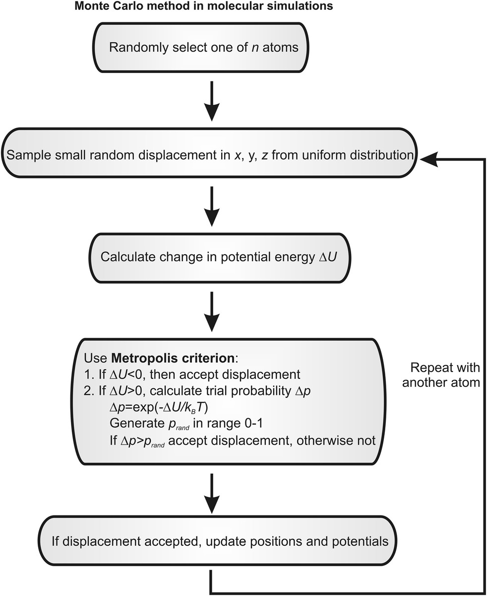
Figure 8.2 Monte Carlo methods in molecular simulations. Simplified schematic of a typical Monte Carlo algorithm for performing stochastic molecular simulations.
This simple process can lead to very complex outputs if, as is generally the case, the biological system is also spatially discretized. That is, probabilistic polling is performed on spatially separated components of the system. This can lead to capturing several emergent properties. Depending on the specific biophysics of the system under study, the incremental time Δt can vary, but has to be small enough to ensure subsaturation levels of Δp that is, Δp < 1 (in practice, Δt is often catered so as to encourage typical values of Δp to be in the range ~0.3–0.5). However, very small values of Δt lead to excessive computational times. Similarly, to get the most biological insight ideally requires the greatest spatial discretization of the system. These two factors when combined can result in requirements of significant parallelization of computation and often necessitate supercomputing, or high performance computing (HPC) resources when applied to molecular simulations. However, there are still several biological processes beyond molecular simulations that can be usefully simulated using nothing more than a few lines of code in any standard engineering software language (e.g., C/C++, MATLAB®, Fortran, Python, LabVIEW) on a standard desktop PC.
A practical issue with the Metropolis criterion is that some microstates during the finite duration of a simulation may be very undersampled or in fact not occupied at all. This is a particular danger in the case of a system that comprises two or more intermediate states of stability for molecular conformations that are separated by relatively large free energy barriers. This implies that the standard Boltzmann factor employed of exp(−ΔU/kBT) is in practice very small if ΔU equates to these free energy barriers. This can result in a simulation being apparently locked in, for example, one very over sampled state. Given enough time of course, a simulation would explore all microstates as predicted from the ergodic hypothesis (see Chapter 6); however, practical computational limitations may not always permit that.
To overcome this problem, a method called “umbrella sampling” can be employed. Here a weighting factor w is used in front of the standard Boltzmann term:
(8.17)Thus, for undersampled states, w would be chosen to be relatively high, and for oversampled states, w would be low, such that all microstates were roughly equally explored in the finite simulation time. Mean values of any general thermodynamic parameter A that can be measured from the simulation (e.g., the free energy change between different conformations) can still be estimated as
(8.18)Similarly, the occupancy probability in each microstate can be estimated using a weighted histogram analysis method, which enables the differences in thermodynamic parameters for each state to be estimated, for example, to explore the variation in free energy differences between the intermediate states.
An extension to Monte Carlo MD simulations is replica exchange MCMC sampling, also known as parallel tempering. In replica exchange, multiple Monte Carlo simulations are performed that are randomly initialized as normal, but at different temperatures. However, using the Metropolis criterion, the molecular configurations at different temperatures can be dynamically exchanged. This results in efficient sampling of high and low energy conformations and can result in improved estimates to thermodynamical properties by spanning a range of simulation temperatures in a computationally efficient way.
An alternative method to umbrella sampling is the simulated annealing algorithm, which can be applied to Monte Carlo as well as other molecular simulations methods. Here the simulation is equilibrated initially at high temperature but then the temperature is gradually reduced. The slow rate of temperature drop gives a greater time for the simulation to explore molecular conformations with free energy levels lower than local energy minima found by energy minimization, which may not represent a global minimum. In other words, it reduces the likelihood for a simulation becoming locked in a local energy minimum.
8.2.4 Ab Initio MD Simulations
Small errors in approximations to the exact potential energy function can result in artifactual emergent properties after long simulation times. An obvious solution is therefore to use better approximations, for example, to model the actual QM atomic orbital effects, but the caveat is an increase in associated computation time. Ab initio MD simulations use the summed QM interatomic electronic potentials UQD experienced by each atom in the system, denoted by a total wave function ψ. Here, UQD is given by the action of Hamiltonian operator Ĥ on ψ (the kinetic energy component of the Hamiltonian is normally independent of the atomic coordinates) and the force FQD by the grad of UQD such that
(8.19)These are, in the simplest cases, again considered as pairwise interactions between the highest energy atomic orbital of each atom. However, since each electronic atomic orbital is identified by a unique value of three quantum numbers, n (the principal quantum number), ℓ (the azimuthal quantum number), and mℓ (the magnetic quantum number), the computation time for simulations scales as ~O(n3). However, Hartree–Fock (HF) approximations are normally applied that reduce this scaling to more like ~O(n2.7). Even so, the computational expense usually restricts most simulations to ~10–100 atom systems with simulation times of ~10–100 ps.
The HF method, also referred to as the self-consistent field method, uses an approximation of the Schrödinger equation that assumes that each subatomic particle, fermions in the case of electronic atomic orbitals, is subjected to the mean field created by all other particles in the system. Here, the n-body fermionic wave function solution of the Schrödinger equation is approximated by the determinant of the n × n spin–orbit matrix called the “Slater determinant.” The HF electronic wave function approximation ψ for an n-particle system thus states
(8.20)The term on the right is the determinant of the spin–orbit matrix. The χ elements of the spin–orbit matrix are the wave functions for the various orthogonal (i.e., independent) wave functions for the n individual particles.
In some cases of light atomic nuclei, such as those of hydrogen, QM MD can model the effects of the atomic nuclei as well as the electronic orbitals. A similar HF method can be used to approximate the total wave function; however, since nuclei are composed of bosons as opposed to fermions, the spin–orbit matrix permanent is used instead of the determinant (a matrix permanent is identical to a matrix determinant, but instead the signs in front of the matrix element product permutations being a mixture of positive and negative as is the case for the determinant, they are all positive for the permanent). This approach has been valuable for probing effects such as the quantum tunneling of hydrogen atoms, a good example being the mechanism of operation of an enzyme called “alcohol dehydrogenase,” which is found in the liver and requires the transfer of an atom of hydrogen using quantum tunneling for its biological function.
Ab initio force fields are not derived from predetermined potential energy functions since they do not assume preset bonding arrangements between the atoms. They are thus able to model chemical bond making and breaking explicitly. Different bond coordination and hybridization states for bond making and breaking can be modeled using other potentials such as the Brenner potential and the reactive force field (ReaxFF) potential.
The use of semiempirical potentials, also known as tight-binding potentials, can reduce the computational demands in ab initio simulations. A semiempirical potential combines the fully QM-based interatomic potential energy derived from ab initio modeling using the spin–orbit matrix representation described earlier. However, the matrix elements are found by applying empirical interatomic potentials to estimate the overlap of specific atomic orbitals. The spin–orbit matrix is then diagonalized to determine the occupancy level of each atomic orbital, and the empirical formulations are used to determine the energy contributions from these occupied orbitals. Tight-binding models include the embedded-atom method also known as the tight-binding second-moment approximation and Finnis–Sinclair model and also include approaches that can approximate the potential energy in heterogeneous systems including metal components such as the Streitz–Mintmire model.
Also, there are hybrid classical and quantum mechanical methods (hybrid QM/MM). Here, for example, classical MD simulations may be used for most of a structure, but the region of the structure where most fine spatial precision is essential is simulated using QM-derived force fields. These can be applied to relatively large systems containing ~104–105 atoms, but the simulation time is limited by QM and thus restricted to simulation times of ~10–100 ps. Examples of this include the simulation of ligand binding in a small pocket of a larger structure and the investigation of the mechanisms of catalytic activity at a specific active site of an enzyme.
8.2.5 Steered MD
Steered molecular dynamics (SMD) simulations, or force probe simulations, use the same core simulation algorithms of either MM or QM simulation methods but in addition apply external mechanical forces to a molecule (most commonly, but not exclusively, a protein) in order to manipulate its structure. A pulling force causes a change in molecular conformation, resulting in a new potential energy at each point on the pulling pathway, which can be calculated at each step of the simulation. For example, this can be used to probe the force dependence on protein folding and unfolding processes, and of the binding of a ligand to receptor, or of the strength of the molecular adhesion interactions between two touching cells. These are examples of thermodynamically nonequilibrium states and are maintained by the input of external mechanical energy into the system by the action of pulling on the molecule.
As discussed previously (see Chapter 2), all living matter is in a state of thermodynamic nonequilibrium, and this presents more challenges in theoretical analysis for molecular simulations. Energy-dissipating processes are essential to biology though they are frequently left out of mathematical/computational models, primarily for three reasons. First, historical approaches inevitably derive from equilibrium formulations, as they are mathematically more tractable. Second, and perhaps most importantly, in many cases, equilibrium approximations seem to account for experimentally derived data very well. Third, the theoretical framework for tackling nonequilibrium processes is far less intuitive than that for equilibrium processes. This is not to say we should not try to model these features, but perhaps should restrict this modeling only to processes that are poorly described by equilibrium models.
Applied force changes can affect the molecular conformation both by changing the relative positions of covalently bonded atoms and by breaking and making bonds. Thus, SMD can often involve elements of both classical and QM MD, in addition to Monte Carlo methods, for example, to poll for the likelihood of a bond breaking event in a given small time interval. The mathematical formulation for these types of bond state calculations relate to continuum approaches of the Kramers theory and are described under reaction–diffusion analysis discussed later in this chapter.
SMD simulations mirror the protocols of single-molecule pulling experiments, such as those described in Chapter 6 using optical and/or magnetic tweezers and AFM. These can be broadly divided into molecular stretches using a constant force (i.e., a force clamp) that, in the experiment, result in stochastic changes to the end-to-end length of the molecule being stretched, and constant velocity experiments, in which the rate of change of probe head displacement relative to the attached molecule with respect to time t is constant (e.g., the AFM tip is being ramped up and down in height from the sample surface using a triangular waveform). If the ramp speed is v and the effective stiffness of the force transducer used (e.g., an AFM tip, optical tweezers) is k, then we can model the external force Fext due to potential energy Uext as
(8.21)where
- t0 is some initial time
Uext can then be summed into the appropriate internal potential energy formulation used to give a revised total potential energy function relevant to each individual atom.
The principal issue with SMD is a mismatch of time scales and force scales between simulation outputs compared to actual experimental data. For example, single-molecule pulling experiments involve generating forces between zero and up to ~10–100 pN over a time scale of typically a second to observe a molecular unfolding event in a protein. However, the equivalent time scale in SMD is more like ~10−9 s, extending as high as ~10−6 s in exceptional cases. To stretch a molecule, a reasonable distance compared to its own length scale, for example, ~10 nm, after ~1 ns of simulation implies a probe ramp speed equivalent to ~10 m s−1 (or ~0.1 Å ps−1 in the units often used in SMD). However, in an experiment, ramp rates are limited by viscous drag effects between the probe and the sample, so speeds equivalent to ~10−6 m s−1 are more typical, seven or more orders of magnitude slower than in the SMD simulations. As discussed in the section on reaction–diffusion analysis later in this chapter, this results in a significantly lower probability of molecular unfolding for the simulations, making it nontrivial to interpret the simulated unfolding kinetics. However, they do still provide valuable insight into the key mechanistic events of importance for force dependent molecular processes and enable estimates to be made for the free energy differences between different folded intermediate states of proteins as a function of pulling force, which provides valuable biological insight.
A key feature of SMD is the importance of water-solvent molecules. Bond rupture, for example, with hydrogen bonds, in particular, is often mediated through the activities of water molecules. The ways in which the presence of water molecules are simulated in general MD are discussed as follows.
8.2.6 Simulating the Effects of Water Molecules and Solvated Ions
The primary challenge of simulating the effects of water molecules on a biomolecule structure is computational. Molecular simulations that include an explicit solvent take into account the interactions of all individual water molecules with the biomolecule. In other words, the atoms of each individual water molecule are included in the MD simulation at a realistic density, which can similarly be applied to any solvated ions in the solution. This generates the most accuracy from any simulation, but the computational expense can be significant (the equivalent molarity of water is higher than you might imagine; see Worked Case Example 8.1).
The potential energy used is typically Lennard–Jones (which normally is only applied to the oxygen atom of the water molecule interacting with the biomolecule) with the addition of the Coulomb potential. Broadly, there are two explicit solvent models: the fixed charge explicit solvent model and the polarizable explicit solvent model. The latter characterizes the ability of water molecules to become electrically polarized by the nearby presence of the biomolecule and is the most accurate physical description but computationally most costly. An added complication is that there are >40 different water models used by different research groups that can account for the electrostatic properties of water (e.g., see Guillot, 2002), which include different bond angles and lengths between the oxygen and hydrogen atoms, different dielectric permittivity values, enthalpic and electric polarizability properties, and different assumptions about the number of interaction sites between the biomolecule and the water’s oxygen atom through its lone pair electrons. However, the most common methods include single point charge (SPC), TIP3P, and TIP4P models that account for most biophysical properties of water reasonably well.
To limit excessive computational demands on using an explicit solvent, periodic boundary conditions (PBCs) are imposed. This means that the simulation occurs within a finite, geometrically well-defined volume, and if the predicted trajectory of a given water molecule takes it beyond the boundary of the volume, it is forced to reemerge somewhere on the other side of the boundary, for example, through the point on the other side of the volume boundary that intersects with a line drawn between the position at which the water molecule moved originally beyond the boundary and the geometrical centroid of the finite volume, for example, if the simulation was inside a 3D cube, then the 2D projection of this might show a square face, with the water molecule traveling to one edge of the square but then reemerging on the opposite edge. PBCs permit the modeling of large systems, though they impose spatial periodicity where there is none in the natural system.
The minimum size of the confining volume of water surrounding the biomolecule needs must be such that it encapsulates the solvation shell (also known as the solvation sphere, also as the hydration layer or hydration shell in the specific case of a water solvent). This is the layer of water molecules that forms around the surface of biomolecules, primarily due to hydrogen bonding between water molecules. However, multiple layers of water molecules can then form through additional hydrogen bond interactions with the primary layer water molecules. The effects of a solvent shell can extend to ~1 nm away from the biomolecule surface, such that the mobility of the water molecules in this zone is distinctly lower than that exhibited in the bulk of the solution, though in some cases, this zone can extend beyond 2 nm. The time scale of mixing between this zone and the bulk solution is in the range 10−15 to 10−12 s and so simulations may need to extend to at least these time scales to allow adequate mixing than if performed in a vacuum. The primary hydration shell method used in classical MD with explicit solvent assumes two to three layers of water molecules and is reasonably accurate.
An implicit solvent uses a continuum model to account for the presence of water. This is far less costly computationally than using an explicit solvent but cannot account for any explicit interactions between the solvent and solute (i.e., between the biomolecule and any specific water molecule). In its very simplest form, the biomolecule is assumed only to interact only with itself, but the electrostatic interactions are modified to account for the solvent by assuming the value of the relative dielectric permittivity term εr in the Coulomb potential. For example, in a vacuum, εr = 1, whereas in water εr ≈ 80.
If the straight-line joining atoms for a pairwise interaction are through the structure of the biomolecule itself, with no accessible water present, then the relative dielectric permittivity for the biomolecule itself should be used, for example, for proteins and phospholipid bilayers, εr can be in the range ~2–4, and nucleic acids ~8; however, there can be considerable variation deepening on specific composition (e.g., some proteins have εr ≈ 20). This very simple implicit solvation model using a pure water solvent is justified in cases where the PMF results in a good approximation to the average behavior of many dynamic water molecules. However, this approximation can be poor in regions close to the biomolecule such as the solvent shell, or in discrete hydration pockets of biomolecules, which almost all molecules in practice have, such as in the interiors of proteins and phospholipid membranes.
The simplest formulation for an implicit solvent that contains dissolved ions is the generalized Born (or simply GB) approximation. GB is semiheuristic (which is a polite way of saying that it only has a physically explicable basis in certain limiting regimes), but which still provides a relatively simple and robust way to estimate long-range electrostatic interactions. The foundation of the GB approximation is the classical Poisson–Boltzmann (PB) model of continuum electrostatics. The PB model uses the Coulomb potential energy with a modified εr value but also considers the concentration distribution of mobile solvated ions. If Uelec is the electrostatic potential energy, then the Poisson equation for a solution of ions can be written as
(8.22)where ρ is the electric charge density. In the case of an SPC, ρ could be modeled as a Dirac delta function, which results in the standard Coulomb potential formulation. However, for spatially distributed ions, we can model these as having an electrical charge dq in an incremental volume of dV at a position r of
(8.23)Applying the Coulomb potential to the interaction between these incremental charges in the whole volume implies
(8.24)The Poisson–Boltzmann equation (PBE) then comes from this by modeling the distribution of ion concentration C as
(8.25)where
- z is the valence of the ion
- qe is the elementary electron charge
- F is the Faraday’s constant
This formulation can be generalized for other types of ions by summing their respective contributions. Substituting Equations 8.23 and 8.24 into Equation 8.25 results in a second-order partial differential equation (PDE), which is the nonlinear Poisson–Boltzmann equation (NLPBE). This can be approximated by the linear Poisson–Boltzmann equation (LPBE) if qeUelec/kBT is very small (known as the Debye–Hückel approximation). Adaptations to this method can account for the effects of counter ions. The LPBE can be solved exactly. There are also standard numerical methods for solving the NLPBE, which are obviously computationally slower than solving the LPBE directly, but the NLPBE is a more accurate electrostatic model than the approximate LPBE.
A compromise between the exceptional physical accuracy of explicit solvent modeling and the computation speed of implicit solvent modeling is to use a hybrid approach of a multilayered solvent model, which incorporates an additional Onsager reaction field potential (Figure 8.3). Here, the biomolecule is simulated in the normal way of QM or MM MD (or both for hybrid QM/MM), but around each molecule, there is a cavity within which the electrostatic interactions with individual water molecules are treated explicitly. However, outside this cavity, the solution is assumed to be characterized by a single uniform dielectric constant. The biomolecule induces electrical polarization in this outer cavity, which in turn creates a reaction field known as the Onsager reaction field. If a NLPBE is used for the implicit solvent, then this can be a physically accurate model for several important properties. However, even so, no implicit solvent model can account for the effects of hydrophobicity (see Chapter 2), water viscous drag effects on the biomolecule, or hydrogen bonding within the water itself.
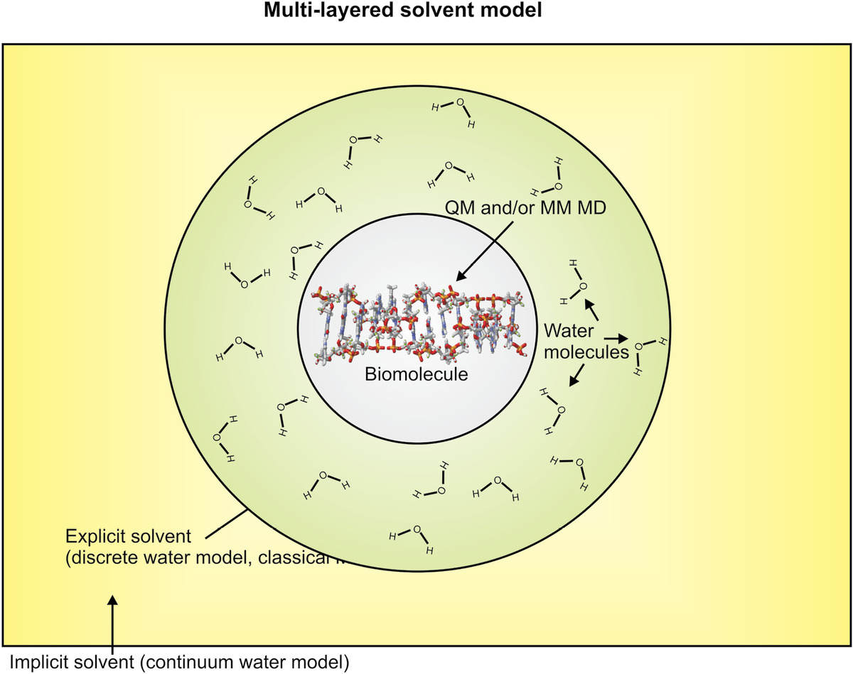
Figure 8.3 Multilayered solvent model. Schematic example of a hybrid molecular simulation approach, here shown with a canonical segment of a Z-DNA (see Chapter 2), which might be simulated using either a QM ab initio method or classical (molecular mechanics) dynamics simulations (MD) approach, or a hybrid of the two, while around it is a solvent shell in which the trajectories of water molecules are simulated explicitly using classical MD, and around this shell is an outer zone of implicit solvent in which continuum model is used to account for the effects of water.
8.2.7 Langevin and Brownian Dynamics
The viscous drag forces not accounted for in implicit solvent models can be included by using the methods of Langevin dynamics (LD). The equation of motion for an atom in an energy potential U exhibiting Brownian motion, of mass m in a solvent of viscous drag coefficient γ, involves inertial and viscous forces, but also a random stochastic element, known as the Langevin force, R(t), embodied in the Langevin equation:
(8.26)Over a long period of time, the mean of the Langevin force is zero but with a finite variance of
The value of γ/m = 1/τ is a measure of the collision frequency between the biomolecule atoms and water molecules, where τ is the mean time between collisions. For example, for individual atoms in a protein, τ is in the range 25–50 ps, whereas for water molecules, τ is ~80 ps. The limit of high γ values is an overdamped regime in which viscous forces dominate over inertial forces. Here τ can for some biomolecule systems in water be as low as ~1 ps, which is a diffusion (as opposed to stochastic) dominated limit called Brownian dynamics. The equation of motion in this regime then reduces to the Smoluchowski diffusion equation, which we will discuss later in this chapter in the section on reaction–diffusion analysis.
One effect of applying a stochastic frictional drag term in LD is that this can be used to slow down the motions of fast-moving particles in the simulation and thus act as feedback mechanism to clamp the particle speed range within certain limits. Since the system temperature depends on particle speeds, this method thus equates to a Langevin thermostat (or equivalently a barostat to maintain the pressure of the system). Similarly, other nonstochastic thermostat algorithms can also be used, which all in effect include additional weak frictional coupling constants in the equation of motion, including the Anderson, isokinetic/Gaussian, Nosé–Hoover, and Berendsen thermostats.
8.2.8 Coarse-Grained Simulation Tools
There are a range of coarse-grained (CG) simulation approaches that, instead of probing the exact coordinates of every single atom in the system independently, will pool together groups of atoms as a rigid, or semirigid, structure, for example, as connected atoms of a single amino acid residue in a protein, or coarser still of groups of residues in a single structural motif in a protein. The forces experienced by the components of biological matter in these CG simulations can also be significantly simplified versions that only approximate the underlying QM potential energy. These reductions in model complexity are a compromise to achieving computational tractability in the simulations and ultimately enable larger length and time scales to be simulated at the expense of loss of fine detail in the structural makeup of the simulated biological matter.
This coarse-graining costs less computational time and enables longer simulation times to be achieved, for example, time scales up to ~10−5 s can be simulated. However, again there is a time scale gap since large molecular conformational changes under experimental conditions can be much slower than this, perhaps lasting hundreds to thousands of microseconds. Further coarse-graining can allow access into these longer time scales, for example, by pooling together atoms into functional structural motifs and modeling the connection between the motifs with, in effect, simple springs, resulting in a simple harmonic potential energy function.
Mesoscale models are at a higher length scale of coarse-graining, which can be applied to larger macromolecular structures. These, in effect, pool several atoms together to create relatively large soft-matter units characterized by relatively few material parameters, such as mechanical stiffness, Young’s modulus, and the Poisson ratio. Mesoscale simulations can model the behavior of macromolecular systems potentially over a time scale of seconds, but clearly what they lack is the fine detail of information as to what happens at the level of specific single molecules or atoms. However, in the same vein of hybrid QM/MM simulations, hybrid mesoscale/CG approaches can combine elements of mesoscale simulations with smaller length scale CG simulations, and similarly hybrid CG/MM simulations can be performed, with the strategy for all these hybrid methods that the finer length scale simulation tools focus on just highly localized regions of a biomolecule, while the longer length scale simulation tool generates peripheral information about the surrounding structures.
Hybrid QM/MM approaches are particularly popular for investigating molecular docking processes. that is, how well or not a small ligand molecule binds to a region of another larger molecule. This process often utilizes relative simple scoring functions to generate rapid estimates for the goodness of fit for a docked molecule to a putative binding site to facilitate fast computational screening and is of specific interest in in silico drug design, that is, using computational molecular simulations to develop new pharmaceutical chemicals.
8.2.9 Software and Hardware for MD
Software evolves continuously and rapidly, and so this is not the right forum to explore all modern variants of MD simulation code packages; several excellent online forums exist that give up-to-date details of the most recent advances to these software tools, and the interested reader is directed to these. However, a few key software applications have emerged as having significant utility in the community of MD simulation research, whose core features have remained the same for the past few years, which are useful to discuss here. Three leading software applications have grown directly out of the academic community, including Assisted Model Building with Energy Refinement (AMBER, developed originally at the Scripps Research Institute, United States), Chemistry at HARvard Macromolecular Mechanics (CHARMM developed at the University of Harvard, United States), and GROningen MAchine for Chemical Simulations (GROMACS, developed at the University of Gröningen, the Netherlands).
The term “AMBER” is also used in the MD community in conjunction with “force fields” to describe the specific set of force fields used in the AMBER software application. AMBER software uses the basic force field of Equation 8.14, with presets that have been parameterized for proteins or nucleic acids (i.e., several of the parameters used in the potential energy approximation have been preset by using prior QM simulation or experimental biophysics data for these different biomolecule types). AMBER was developed for classical MD, but now has interfaces that can be used for ab initio modeling and hybrid QM/MM. It includes implicit solvent modeling capability and can be easily implemented on graphics processor units (GPUs, discussed later in this chapter). It does not currently support standard Monte Carlo methods but has replica exchange capability.
CHARMM has much the same functionality as AMBER. However, the force field used has more complexity, in that it includes additional correction factors:
(8.27)The addition of the impropers potential (Uimpropers) is a dihedral correction factor to compensate for out-of-plane bending (e.g., to ensure that a known planar structural motif remains planar in a simulation) with kω being the appropriate impropers stiffness and ω is the out-of-pane angle deviation about the equilibrium angle ωeq˙ The Urey–Bradley potential (UU-B) corrects for cross-term angle bending by restraining the motions of bonds by introducing a virtual bond that counters angle bending vibrations, with u a relative atomic distance from the equilibrium position ueq. The CHARMM force field is physically more accurate than that of AMBER, but at the expense of greater computational cost, and in many applications, the additional benefits of the small correction factors are marginal.
GROMACS again has many similarities to AMBER and CHARMM but is optimized for simulating biomolecules with several complicated bonded interactions, such as biopolymers in the form of proteins and nucleic acids, as well as complex lipids. GROMACS can operate with a range of force fields from different simulation software including CHARMM, AMBER, and CG potential energy functions; in addition, its own force field set is called Groningen molecular simulation (GROMOS). The basic GROMOS force field is similar to that of CHARMM, but the electrostatic potential energy is modeled as a Coulomb potential with reaction field (UCRF), which in its simplest form is the sum of the standard ~1/rij Coulomb potential (UC) with additional contribution from a reaction field (URF), which represents the interaction of atom i with an induced field from the surrounding dielectric medium beyond a predetermined cutoff distance Rrf due to the presence of atom j:
(8.28)where
- ε1 and ε2 are the relative dielectric permittivity values inside and outside the cutoff radius, respectively
- κ is the reciprocal of the Debye screening length of the medium outside the cutoff radius
The software application NAMD (Nanoscale Molecular Dynamics, developed at the University of Illinois at Urbana-Champaign, United States) has also recently emerged as a valuable molecular simulation tool. NAMD benefits from using a popular interactive molecular graphics rendering program called “visual molecular dynamics” (VMD) for simulation initialization and analysis, but its scripting is also compatible with other MD software applications including AMBER and CHARMM and was designed to be very efficient at scaling simulations to hundreds of processors on high-end parallel computing platforms, incorporating Ewald summation methods. The standard force field used is essentially that of Equation 8.14. Its chief popularity has been for SMD simulations, for which the setup of the steering conditions are made intuitive through VMD.
Other popular packages include those dedicated to more niche simulation applications, some commercial but many homegrown from academic simulation research communities, for example, ab initio simulations (e.g., CASTEP, ONETEP, NWChem, TeraChem, VASP), CG approaches (e.g., LAMMPS, RedMD), and mesoscale modeling (e.g., Culgi). CG tools of oxDNA and oxRNA have utility in mechanical and topological CG simulations of nucleic acids. Others for specific docking processes can be simulated (e.g., ICM, SCIGRESS) and molecular design (e.g., Discovery studio, TINKER) and folding (e.g., Abalone, fold.it, FoldX), with various valuable molecular visualization tools available (e.g., Desmond, VMD).
The physical computation time for MD simulations can take anything from a few minutes for a simple biomolecule containing ~100 atoms up to several weeks for the most complex simulations of systems that include up to ~10,000 atoms. Computational time has improved dramatically over the past decade however due to four key developments:
- CPUs have got faster, with improvements to miniaturizing the effective minimum size of a single transistor in a CPU (~40 nm, at the time of writing) enabling significantly more processing power. Today, CPUs typically contain multiple cores. A core is an independent processing unit of a CPU, and even entry-level PCs and laptops use a CPU with two cores (dual-core processors). More advanced computers contain 4–8 core processors, and the current maximum number of cores for any processor is 16. This increase in CPU complexity is broadly consistent with Moore’s law (Moore, 1965). Moore’s law was an interpolation of reduction of transistor length scale with time, made by Gordon E. Moore, the cofounder of Intel, in which the area density of transistors in densely packed integrated circuits would continue to roughly double every two years. The maximum size of a CPU is limited by heat dissipation considerations (but this again has been improved recently by using CPU circulating cooling fluids instead air cooling). The atomic spacing of crystalline silicon is ~0.5 nm that may appear to place an ultimate limit on transistor miniaturization; however, there is increasing evidence that new transistor technology based on smaller length scale quantum tunneling may push the size down even further.
- Improvements in simulation software have enabled far greater parallelizability to simulations, especially to route parallel aspects of simulations to different cores of the same CPU, and/or to different CPUs in a network cluster of computers. There is a limit, however, to how much of a simulation can be efficiently parallelized, since there are inevitably bottlenecks due to one parallelized component of the simulation having to wait for the output from another before it can proceed, though of course multiple different simulations can be run simultaneously at least, for example, for simulations that are stochastic in nature and so are replicated independently several times or trying multiple different starting conditions for deterministic simulations.
- Supercomputing resources have improved enormously, with dedicated clusters of ultrafast multiple-core CPUs coupled with locally dedicated ultrahigh bandwidth networks. The use of academic research supercomputers is in general extended to several users where supercomputing time is allocated to enable batch calculations in a block and can be distributed to different computer nodes in the supercomputing cluster.
- Recent developments in GPU technology have revolutionized molecular simulations. Although the primary function of a GPU is to assist with the rendering of graphics and visual effects so that the CPU of a computer does not have to, a modern GPU has many features that are attractive to brute number-crunching tasks, including molecular simulations. In essence, CPUs are designed to be flexible in performing several different types of tasks, for example, involving communicating with other systems in a computer, whereas GPUs have more limited scope but can perform basic numerical calculations very quickly. A programmable GPU contains several dedicated multiple-core processors well suited to Monte Carlo methods and MD simulations with a computational power far in excess of a typical CPU. Depending on the design, a CPU core can execute up to 8× 32 bit instructions per clock cycle (i.e., 256 bit per clock cycle), whereas a fast GPU used for 3D video-gaming purposes can execute ~3200× 32 bit instructions per clock, a bandwidth speed difference of a factor of ~400. A very-high-end CPU of, for example, having ~12 cores, has a higher clock rate of up to 2–3 GHz versus 0.7–0.8 GHz for GPUs, but even comparing coupling together four such 12-core CPUs, a single reasonable gaming GPU is faster by at least a factor of 5 and, at the time of writing, cheaper by a factor of at least an order of magnitude. GPUs can now be programmed relatively easily to perform molecular simulations, outperforming more typical multicore CPUs by a speed factor of ~100. GPUs have now also been incorporated into supercomputing clusters. For example, the Blue Waters supercomputer at the University of Urbana-Champaign is, as I write, the fastest supercomputer on any university campus and indeed one of the fastest supercomputers in the world, which can use four coupled GPUs that have performed a VMD calculation of the electrostatic potential for one frame of a MD simulation of the ribosome (an enormously complex biological machine containing over 100,000 atoms with a large length scale of a few tens of nm; see Chapter 2) in just 529 s using just one of these available GPUs, as opposed to ~5.2 h using on a single ultrafast CPU core.
The key advantage with GPUs is that they currently offer better performance per dollar than several of high-end CPU core applied together in a supercomputer, either over a distributed computer network or clustered together in the same machine. A GPU can be installed on an existing computer and may enable larger calculations for less money than building a cluster of computers. However, several supercomputing clusters have GPU nodes now. One caveat is that GPUs do not necessarily offer good performance on any arbitrary computational task, and writing code for a GPU can still present issues with efficient memory use.
One should also be mindful of the size of the computational problem and whether a supercomputer is needed at all. Supercomputers should really be used for very large jobs that no other machine can take on and not be used to make a small job run a bit more quickly. If you are running a job that does not require several CPU cores, you should really use a smaller computer; otherwise, you would just be hogging resources that would be better spent on something else. This idea is the same for all parallel computing, not just for problems in molecular simulation.
Another important issue to bear in mind is that for supercomputing resources you usually have a queue to wait in for your job to start on a cluster. If you care about the absolute time required to get an output from a molecular simulation, the real door-to-door time if you like, it may be worth waiting longer for a calculation to run on a smaller machine in order to save the queue time on a larger one.
8.2.10 Ising Models
The Ising model was originally developed from quantum statistical mechanics to explain the emergent properties of ferromagnetism (see Chapter 5) by using simple rules of local interactions between spin-up and spin-down states. These localized cooperative effects result in emergent behavior at the level of the whole sample. For example, the existence of either ferromagnetic (ordered) or paramagnetic (disordered) bulk emergent features in the sample, and phase transition behavior between the two bulk states, which is temperature dependent up until a critical point (in this example known as the Curie temperature). Many of the key features of cooperativity between smaller length scale subunits, leading to a different larger length scale emergent behavior are also present in the Monod–Wyman–Changeux (MWC) model, also known as the symmetry model, which describes the mechanism of cooperative ligand binding in some molecular complexes, for example, the binding of oxygen to the tetramer protein complex hemoglobin (see Chapter 2), as occurs inside red blood cells for oxygenating tissues.
In the MWC model, the phenomenon is framed in terms of allostery; that is, the binding of one subunit affects the ability of it and/or others in the complex to bind a ligand molecule, in which biochemists often characterize by the more heuristic Hill equation for the fraction θ of bound ligand at concentration C that has a dissociation rate constant of Kd (see Chapter 7):
(8.29)where n is the empirical Hill coefficient such that n = 1 indicates no cooperativity, n < 1 is negatively cooperative, and n > 1 is positively cooperative.
Hemoglobin has a highly positive cooperativity with n = 2.8 indicating that 2–3 of the 4 subunits in the tetramer interact cooperatively during oxygen binding, which results in a typically sigmoidal shaped all-or-nothing type of response if θ is plotted as a function of oxygen concentration. However, the Ising model puts this interaction on a more generic footing by evoking the concept of an interaction energy that characterizes cooperativity and thus can be generalized into several systems, biological and otherwise.
In the original Ising model, the magnetic potential energy of a sample in which the ith atom has a magnetic moment (or spin) σi is given by the Hamiltonian equation:
(8.30)where K is a coupling constant with the first term summation over adjacent atoms with magnetic moments of spin +1 or −1 depending on whether they are up or down and B is an applied external magnetic field. The second term is an external field interaction energy, which increases the probability for spins to line up with the external field to minimize this energy. One simple prediction of this model is that at low B the nearest-neighbor interaction energy will bias nearest neighbors toward aligning with the external field, and this results in clustering of aligned spins, or conformational spreading in the sample of spin states (Figure 8.4a).
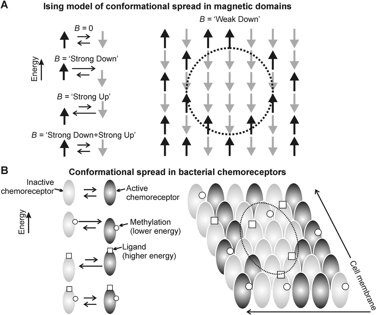
Figure 8.4 Ising modeling in molecular simulations. (a) Spin-up (black) and spin-down (gray) of magnetic domains at low density in a population are in thermal equilibrium, such that the relative proportion of each state in the population will change as expected by the imposition of a strong external magnetic B-field, which is either parallel (lower energy) or antiparallel (higher energy) to the spin state of the magnetic domain (left panel). However, the Ising model of statistical quantum mechanics predicts an emergent behavior of conformational spreading of the state due to an interaction energy between neighboring domains, which results in spatial clustering of one state in a densely packed population as occurs in a real ferromagnetic sample, even in a weak external magnetic field (dashed circle right panel). (b) A similar effect can be seen for chemoreceptor expressed typically in the polar regions of cell membranes in certain rodlike bacteria such as Escherichia coli. Chemoreceptors are either in an active conformation (black), which results in transmitting the ligand detection signal into the body of the cell or an inactive conformation (gray) that will not transmit this ligand signal into the cell. These two states are in dynamic equilibrium, but the relative proportion of each can be biased by either the binding of the ligand (raises the energy state) or methylation of the chemoreceptor (lowers the energy state) (left panel). The Ising model correctly predicts an emergent behavior of conformational spreading through an interaction energy between neighboring chemoreceptors, resulting in clustering of the state on the surface of the cell membrane (dashed circle, right panel).
This same general argument can be applied to any system that involves a nearest-neighbor interaction between components that exist in two states of different energy, whose state can be biased probabilistically by an external field of some kind. At the long biological length scale, this approach can characterize flocking in birds and swarming in insects and even of social interactions in a population, but at the molecular length scale, there are several good exemplars of this behavior too. For example, bacteria swim up a concentration gradient of nutrients using a mechanism of a biased random walk (see later in this chapter), which involves the use of chemoreceptors that are clustered over the cell membrane. Individual chemoreceptors are two stable conformations, active (which can transmit the detected signal of a bound nutrient ligand molecule to the inside of the cell) and inactive (which cannot transmit the bound nutrient ligand signal to the inside of the cell). Active and inactive states of an isolated chemoreceptor have the same energy. However, binding of a nutrient ligand molecule lowers the energy of the inactive state, while chemical adaptation (here in the form of methylation) lowers the energy of the active state (Figure 8.4b, left panel).
However, in the cell membrane, chemoreceptors are tightly packed, and each in effect interacts with its four nearest neighbors. Because of steric differences between the active and inactive states, its energy is lowered by every neighboring chemoreceptor that is in the same conformational state but raised by every neighboring receptor in the different state. This interaction can be characterized by an equivalent nearest-neighbor interaction energy (see Shi and Duke, 1998), which results in the same sort of conformational spreading as for ferromagnetism, but now with chemoreceptors on the surface of cell membranes (Figure 8.4b, right panel), and this behavior can be captured in Monte Carlo simulations (Duke and Bray, 1999) and can be extended to molecular systems with more challenging geometries, for example, in a 1D ring of proteins as found in the bacterial flagellar motor (Duke et al., 2001).
This phenomenon of conformational spreading can often be seen in the placement of biophysics academics at conference dinners, if there is a “free” seating arrangement. I won’t go into the details of the specific forces that result in increased or decreased energy states, but you can use your imagination.
8.3 Mechanics of Biopolymers
Many important biomolecules are polymers, for example, proteins, nucleic acids, lipids, and many sugars. Continuum approaches of polymers physics can be applied to many of these molecules to infer details concerning their mechanical properties. These include simple concepts such as the freely jointed chain (FJC) and freely rotating chain (FRC) with approximations such as the Gaussian chain (GC) and wormlike chain (WLC) approaches and how these entropic spring models predict responses of polymer extension to imposed force. Nonentropic sources of biopolymer elasticity to model less idealized biopolymers are also important. These methods enable theoretical estimates of a range of valuable mechanical parameters to be made and provide biological insight into the role of many biopolymers.
8.3.1 Discrete Models for Freely Jointed Chains and Freely Rotating Chains
The FJC model, also called the “random-flight model” or “ideal chain,” assumes n infinitely stiff discrete chain segments each of length b (known as the Kuhn length) that are freely jointed to, and transparent to, each other (i.e., parts of the chain can cross through other parts without impediment) such that the directional vector ri of the ith segment is uncorrelated with all other segments (Figure 8.5a). The end-to-end distance of the chain R is therefore equivalent to a 3D random walk. We can trivially deduce the first moment of the equivalent vector R (the time average over a long time) as
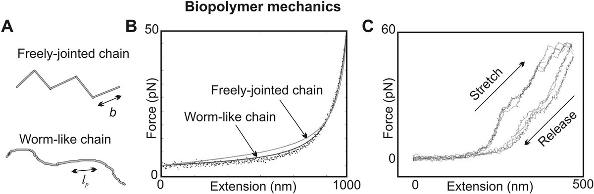
Figure 8.5 Modeling biopolymer mechanics. (a) Schematic of freely jointed and wormlike chains (WLCs) indicating Kuhn (b) and persistence lengths (lp), respectively. (b) Typical fits of WLC and freely jointed chain models to real experimental data obtained using optical tweezers stretching of a single molecule of the muscle protein titin (dots), which (c) can undergo hysteresis due to the unfolding of domains in each structure. (Data courtesy of Mark Leake, University of York, York, UK).
Since there is no directional bias to ri. The second moment of R (the time average of the dot-product R2 over long time) is similarly given by
(8.32)The last term equates to zero since ri · rj is given by rirj cos θij where θij is the angle between the segment vectors, and
So the root mean square (rms) end-to-end distance scales simply with
Another valuable straightforward result also emerges for the radius of gyration of the FJC, which is the mean square distance between all of the segments in the chain. This is identical to the mean distance of the chain from its center of mass, denoted by vector RG:
(8.35)
Using the result of Equation 8.34, we can then say
(8.36)A valuable general approximation comes from using high values of n in this discrete equation or by approximating the discrete summations as continuum integrals, which come to the same result of
(8.37)Another useful result that emerges from similar analysis is the case of the radius of gyration of a branched polymer, where the branches are of equal length and joined at a central node such that if there are f such branches, the system is an f arm star polymer. This result is valuable for modeling biopolymers that form oligomers by binding together at one specific end, which can be reduced to
(8.38)The first and second terms represent inter- and intra-arm contributions respectively, which can be evaluated as
(8.39)Thus, at small f (= 1 or 2), α is 1, for much larger f, α is ~3/f and RG f-arm decreases roughly as ~3RG/f The FRC has similar identical stiff segment assumptions as for the FJC; however, here the angle θ between position vectors of neighboring segments is fixed but the torsional angle ψ (i.e., the angle of twist of one segment around the axis of a neighboring segment) is free to rotate. A similar though slightly more involved analysis to that of the FJC, which considers the recursive relation between adjacent segments, leads to
(8.40)For high values of n, this equation can be reduced to the approximation
(8.41)This additional angular constraint often results in better agreement to experimental data, for example, using light scattering measurements from many proteins (see Chapter 3) due to real steric constraints due to the side groups of amino acid residues whose effective value of g is in the range ~2–3.
8.3.2 Continuum Model for the Gaussian Chain
The GC is a continuum approximation of the FJC (which can also be adapted for the FRC) for large n (>100), applying the central limit theorem to the case of a 1D random walk in space. Considering n unitary steps taken on this random walk that are parallel to the x-axis, a general result for the probability p(n, x) for being a distance x away from the origin, which emerges from Stirling’s approximation to the log of the binomial probability density per unit length at large n, is
(8.42)This integral is evaluated using as a standard Gaussian integral. Thus, we can say
(8.43)However, a FJC random walk is in 3D, and so the probability density per unit volume p(n, R) is the product of the three independent probability distributions in x, y, and z, and each step is of length b, leading to
(8.44)For example, the probability of finding the end of the polymer in a spherical shell between R and R + dR is then p(n, R) · 4πR2dR. This result can be used to predict the effective hydrodynamic (or Stokes) radius (RH). Here, the effective rate of diffusion of all arbitrary sections between the ith and jth segments is additive, and since the diffusion coefficient is proportional to the reciprocal of the effective radius of a diffusing particle from the Stokes–Einstein equation (Equation 2.12), this implies
(8.45)
Thus
8.3.3 Wormlike Chains
Biopolymers with relatively long segment lengths are accurately modeled as a wormlike chain, also known as the continuous version of the Kratky–Porod model. This model can be derived from the FRC by assuming small θ, with the result that
(8.46)where
lp is known as the persistence length
Rmax is the maximum end-to-end length, which is equivalent to the contour length from the FJC of nb
In the limit of a very long biopolymer (i.e., Rmax ≫ lp),
(8.47)This is the ideal chain limit for a relatively compliant biopolymer. Similarly, in the limit of a short biopolymer (i.e., Rmax ≪ lp),
(8.48)This is known as the rodlike limit corresponding to a very stiff biopolymer.
8.3.4 Force Dependence of Polymer Extension
The theory of flexible polymers described previously for biopolymer mechanics results in several different polymer conformations having the same free energy state (i.e., several different microstates). At high end-to-end extension close to a biopolymer’s natural contour length, there are fewer conformations that the molecule can adopt compared to lower values. Therefore, there is an entropic deficit between high and low extensions, which is manifest as an entropic force in the direction of smaller end-to-end extension.
The force response F of a biopolymer to a change in end-to-end extension r can be characterized in the various models of elasticity described earlier. If the internal energy of the biopolymer stays the same for all configurations (in other words that each segment in the equivalent chain is infinitely rigid), then entropy is the only contribution to the Helmholtz free energy A:
(8.49)where p is the radial probability density function discussed in the previous section. The restoring force experienced by a stretched molecule of end-to-end length R is then given by
(8.50)with a molecular stiffness k given by
(8.51)Using the result for p for the GC model of Equation 8.44 indicates
(8.52)Therefore, the GC restoring force is given by
(8.53)Thus, the GC molecular stiffness is given by
(8.54)This implies that a GC exhibits a constant stiffness with extension, that is, it obeys Hooke’s law, with the stiffness proportional to the thermal energy scale of kBT and to the reciprocal of b2. This is a key weakness with the GC model; a finite force response even after the biopolymer is stretched beyond its own contour length is clearly unphysical. The FJC and WLC models are better for characterizing a biopolymer’s force response with extension. Evaluating p for the FJC and WLC models is more complicated, but these ultimately indicate that, for the FJC model,
(8.55)Similarly, for the WLC model,
(8.56)The latter formulation is most popularly used to model force-extension data generated from experimental single-molecule force spectroscopy techniques (see Chapter 6), and this approximation deviates from the exact solution by <10% for forces <100 pN. Both models predict a linear Hookean regime at low forces. Examples of both FJC and WLC fit to the same experimental data obtained from optical tweezers stretching of a single molecule of titin are shown in Figure 8.5b.
By integrating the restoring force with respect to end-to-end extension, it is trivial to estimate the work done, ΔW in stretching a biopolymer from zero up to end-to-end extension R. For example, using the FJC model, at low forces (F < kBT/b and R < Rmax/3),
(8.57)In other words, the free energy cost per spatial dimension degree of freedom reaches kBT/2 when the end-to-end extension reaches its mean value. This is comparable to the equivalent energy E to stretch an elastic cylindrical rod of radius r modeled by Hooke’s law:
(8.58)where
Y is the Young’s modulus
σ is the stress F/πr2
F0 is πr2Y
However, at high forces and extensions, the work done becomes
(8.59)where C is a constant. As the biopolymer chain extension approaches its contour length Rmax, the free energy cost in theory diverges.
8.3.5 Real Biopolymers
As discussed earlier, the GC chain model does not account well for the force response of real molecules to changes in molecular extension, which are better modeled by FJC, FRC, and WLC models. In practice, however, real biopolymers may have heterogeneity in b and lp values, that is, there can be multiple different structural components within a molecule. We can model these effects in the force dependence as having N-such separate chains attached in parallel, both with FJC and WLC models. Thus, for N-FLC,
(8.60)Similarly, for N-WLC,
(8.61)However, in practice, real biopolymers do not consist of segments that are freely jointed as in the FJC. There is real steric hindrance to certain conformations that are not accounted for in the FJC model, though to some extent these can be modeled by the additional angular constraints on the FRC model, which are also embodied in the WLC model. However, all of these models have the key assumption that different sections of the molecule can transparently pass through each other, which is obviously unphysical. More complex excluded volume WLC approaches can disallow such molecular transparency.
Also, the assumption that chain segments, or equivalent sections of the chain of lp length scale, are infinitely stiff is unrealistic. In general, there may also be important enthalpic spring contributions to molecular elasticity. For example, the behavior of the chain segments can be more similar to Hookean springs, consistent with an increasing separation of constituent atoms with greater end-to-end distance, resulting in an opposing force due to either bonding interactions (i.e., increasing the interatomic separation beyond the equilibrium value, similarly for bond angle and dihedral components) and for nonbonding interactions, for example, the Lennard–Jones potential predicts a smaller repulsive force and greater vdW attractive force at increasing interatomic separations away from the equilibrium separation, and similar arguments apply to electrostatic interactions. These enthalpic effects can be added to the purely entropic components in modified elastically jointed chain models. For example, for a modified FJC model in which a chain is composed of freely jointed bonds that are connected by joints with some finite total enthalpic stiffness K,
(8.62)or similarly, for an enthalpic-modified WLC model,
(8.63)Deviations exist between experimentally determined values of b and lp parameters and those predicted theoretically on the basis of what appear to be physically sensible length scales for known structural information. For example, the length of a single amino acid in a protein, or the separation of a single nucleotide base pair in a nucleic acid, might on first inspection seem like sensible candidates for an equivalent segment of a chain. Also, there are inconsistencies between experimentally estimated values for RG of some biopolymers compared against the size of cellular structures that contain these molecules (Table 8.1).
| Molecule | Number of Nucleotides or Amino Acids | Contour Length | b | Ip | RG | Confining Structure | ||||||
|---|---|---|---|---|---|---|---|---|---|---|---|---|
| dsDNA; λ virus | 49,000 | 15,000 | 100 nm | 50 nm | 0.5 μm | 60 nm; capsid diameter | ||||||
| dsDNA; T2 virus | 150,000 | 50,000 | 100 nm | 50 nm | 900 | 100 nm; capsid diameter | ||||||
| dsDNA; E coli bacteria | 4.6 × 10⁶ | 15 mm | 100 nm | 50 nm | 5 μm | 1–2 μm; cell width–length | ||||||
| dsDNA; human | 4 × 10⁹ | 2 m | 100 nm | 50 nm | 0.2 mm | 5–6 μm; nucleus diameter | ||||||
| ssDNA; STMV virus | 1,063 | 0.7 μm | 0.6 nm | 2 nm | 15 nm | 7 nm; capsid diameter | ||||||
| Titin protein; Human muscle | 30,000 | 1.7 μm | 4 nm | 2 nm | 30 nm | 3 nm; titin spacing | ||||||
| Titin protein; “random coil” | 1,100 | 0.7 μm | 0.4 nm | 0.5 nm | 5 nm | 3 nm; titin spacing |
The persistence length values of typical biopolymers can vary from as low as ~0.2 nm (equivalent to a chain segment length of ~0.4 nm, which is the same as the length of a single amino acid residue) for flexible molecules such as denatured proteins and single-stranded nucleic acids, through tens of nanometers for stiffer molecules such as double-stranded DNA, up to several microns for very stiff protein filaments (e.g., the F-actin filament in muscle tissue has a persistence length of ~15 μm). The general trend for real biopolymers is that the estimated RG is often much larger than the length scale of the cellular “container” of that molecule. This implies the presence of significant confining forces beyond just the purely entropic spring forces of the biomolecules themselves. These are examples of out of thermal equilibrium behavior and so require an external free energy input from some source to be maintained.
Deviations to models based on the assumption can also occur in practice due to repulsive self-avoidance forces (i.e., excluded volume effects) but also to attractive forces between segments of the biopolymer chain in the case of a poor solvent (e.g., hydrophobic-driven interactions). Flory’s mean field theory can be used to model these effects. Here, the radius of gyration of a polymer relates to n through the Flory exponent υ as RG ~ nυ. In the case of a so-called theta solvent, the polymer behaves as an ideal chain and υ = ½. In reality, the solvent is somewhere between extremes of being a good solvent (results in additional repulsive effects between segments such that the polymer conformation is an excluded volume coil) and υ = 3/5 and a bad solvent (the polymer is compacted to a sphere) and υ = 1/3.
In practice, the realistic modeling of biopolymer mechanics may involve not just the intrinsic force response of the biopolymer but also the effects of external forces derived from complicated potential energy functions, more similar to the approach taken for MD simulations (see earlier in this chapter). For example, modeling the translocation of a polymer through a nanopore, a common enough biological process, is nontrivial. The theoretical approaches that agree best with experimental data involve MD simulations combined with biopolymer mechanics, and the manner in which these simulations are constructed illustrates the general need for exceptionally fine precision not only in experimental measurement but in theoretical analysis also at this molecular level of biophysical investigation.
Here, the polymer is typically modeled as either an FJC or WLC, but then a nontrivial potential energy function U is constructed corresponding to the summed effects from each segment, including contributions from a segment-bonding potential, chain bending, excluded volume effects due to the physical presence of the polymer itself not permitting certain spatial conformations, electrostatic contributions, and vdW effects between the biopolymer and nanopore wall. Then, the Langevin equation is applied that equates the force experienced by any given segment to the sum of the grad of U with an additional contribution due to random stochastic coupling to the water solvent thermal bath. By then, solving this force equation for each chain segment in ~10−15 s time step predictions can be made as to position and orientation of each given segment as a function of time, to simulate the translocation process through the nanopore.
The biophysics of a matrix of biopolymers adds a further layer of complication to the theoretical analysis. This is seen, for example, in hydrogels, which consist of an aqueous network of concentrated biopolymers held together through a combination of solvation and electrostatic forces and long range vdW interactions. However, some simple power-law analysis makes useful predications here as to the variation of the elastic modulus G of a gel that varies as ~C2.25, where C is the biopolymer concentration, which illustrates a very sensitive dependence to gel stiffness for comparatively small changes in C (much of the original analytical work in this area, including this, was done by one of the pioneers of biopolymer mechanics modeling, Pierre Gilles de Gennes).
8.3.6 Modeling Biomolecular Liquid–Liquid Phase Separation
A recent emergence of myriad experimental studies of biomolecular liquid–liquid phase separation (LLPS, see Chapter 2) has catalyzed the development of new models to investigate how LLPS droplets form and are regulated. The traditional method to investigate liquid–liquid phase separation is Flory–Huggins solution theory, which models the dissimilarity in molecular sizes in polymer solutions taking into account the entropic and enthalpic changes that drive the free energy of mixing. It uses a random walk approach for polymer molecules on a lattice. To obtain the free energy, you need calculate the interaction energies for a given lattice square with its nearest neighbors, which can therefore involve “like” interactions such as polymer–polymer and solvent–solvent, or “unlike” interactions of polymer–solvent.
During phase separation, demixing results in an increase in order in reducing the number of available thermodynamic microstates in the system, thus a decrease in entropy. Therefore, the driving force in phase separation is the net gain in enthalpy that can occur in allowing like polymer and solvent molecules to interact, and much of modern theory research into LLPS lies in trying to understand specifically what causes this imbalance between entropic loss and enthalpic gain. For computational simplicity, a mean-field treatment is often used, which generates an average forcefield across the lattice to account for all neighbor effects. Flory–Huggins theory and its variants can be used to fit data from a range of experiments and construct phase diagrams, for example to predict temperature boundaries at which phase separation can occur and providing semi-quantitative explanations for the effects of ionic strength and sequence dependence of RNA and proteins have on the shape of these phase diagrams.
One weakness with traditional Flory–Huggins theory is that it fails to predict an interesting feature of real biomolecular LLPS in live cells, that droplets have a preferred length scale—Flory–Huggins theory predicts that either side of a boundary on the phase transition diagram a phase transition ultimately either completely mixes or, in the super-saturation side of the boundary, demixes completely after a sufficiently long time such that ultimately all of the polymer material will phase separate—in essence resulting in two physically separated states of just polymer and solvent; in other words, this would be manifest as one very large droplet inside a cell were it to occur. However, what is observed in general is a range of droplet diameters typically from a few tens of nanometers up to several hundred nanometers. One approach to account for this distribution and preferment of length scale involves modeling the effects of surface tension in droplet growth embodied in the classical nucleation Szilard model, which allows reversible transitions to occur between droplets of different size as they exchange material through diffusion, both through droplets growing (or “ripening”) and shrinking.
For a simple theoretical treatment of this effect, if N is the number of biomolecules phase separated into a droplet, then the free energy ΔG in the super-saturated regime can be modeled as –AN + BN2/3 where A and B are positive constants that depend upon the enthalpic of interaction and energy per unit area at the interface between the droplet and the surrounding water solvent due to surface tension (see Worked Case Example 8.3). This results in a maximum value ΔGmax as a function of N, which thus serves as a nucleation activation barrier; from ΔG in the range 0–ΔGmax, the effect from surface tension slows down the rate of droplet growth, whereas above ΔGmax, droplet growth is less impaired by surface tension and more dominated by the net gain in enthalpy, at the expense of depleting the population of smaller droplets (this process is known as Ostwald ripening (also known as coarsening) and is a signature of liquid–liquid phase transitions).
Sviliard modeling can explain the qualitative appearance of size distributions of droplets, but it does not explain what drives the fine-tuning of the A and B parameters, which is down to molecular scale interaction forces. A valuable modeling approach which has emerged to address these questions has involved a stickers-and-spacers framework that has been adapted from the field of interacting polymers (Choi et al., 2020). This approach models interacting polymers as strings which contain several sticker regions separated by noninteracting spacer sequences, such that the spacers can undergo spatial fluctuations to enable interactions between stickers either from the same molecule or with neighbors. Stickers are defined at specific locations of the molecule due to the likelihood of electrostatic or hydrophobic interactions (which are dependent on the nature of the sequence of the associated polymer, typically either RNA or a peptide) to enable insight into how multivalent proteins and RNA molecules can drive phase transitions that give rise to biomolecular condensates. The reduction in complexity in modeling a polymer as a string with sticky regions avails the approach to coarse-graining computation and so has been very successful in simulating how droplets form over relatively extended durations of several microseconds even for systems containing many thousands of molecules.
8.4 Reaction, Diffusion, and Flow
Reaction–diffusion continuum mathematical models can be applied to characterize systems that involve a combination of chemical reaction kinetics and mobility through diffusional processes. This covers a wide range of phenomena in the life sciences. These mathematical descriptions can sometimes be made more tractable by first solving in the limits of being either diffusion limited (i.e., fast reaction kinetics, slow diffusion) or reaction limited (fast diffusion, slow reaction kinetics), though several processes occur in an intermediate regime in which both reaction and diffusion effects need to be considered. For example, the movement of molecular motors on tracks in general comprises both a random 1D diffusional element and a chemical reaction element that results in bias of the direction of the motor motion on the track. Other important continuum approaches include methods that characterize fluid flow in and around the biological structures.
8.4.1 Markov Models
The simplest general reaction–diffusion equation that considers the spatial distribution of the localization probability P of a biomolecule as a function of time t at a given point in space is as follows:
(8.64)The first term on the right-hand side of the equation is the diffusional term, with D being the diffusion coefficient. The second term v can often be a complicated function that embodies the reaction process. The form of the reaction–diffusion equation that describes Brownian diffusion of a particle in the presence of an external force (the reaction element) is also known as the Smoluchowski equation or Fokker–Planck equation (also sometimes referred to as the Kolmogorov equation), all of which share essentially the same core features in the mathematical modeling of Markov processes; as discussed previously in the context of localization microscopy (see Chapter 4), these processes are memoryless or history independent. Here, the function v is given by an additional drift drag component due to the action of an external force F on a particle of viscous drag coefficient γ, and the Fokker–Planck equation in 1D becomes
(8.65)An example of such a reaction–diffusion process in biology is the movement of molecular motors on tracks, such as the muscle protein myosin moving along an F-actin filament, since they can diffuse randomly along the 1D but experience an external force due to the power stroke action of the myosin on the F-actin while a motor is in a given active state. However, in addition to this mechanical component, there is also a chemical reaction component that involves transitions into and out of a given active state of the motor. For example, if the active state of a motor is labeled as i, and a general different state is j, then the full reaction–diffusion equation becomes the Fokker–Planck equation plus the chemical transition kinetics component:
(8.66)where kij and kji are the equivalent off-rates from state i to j, and on-rates from state j to i, respectively. Most PDEs of reaction–diffusion equations are too complicated to be solved analytically. However, the model of the process of a single molecular motor, such as myosin, translocating on a track, such as F-actin, can be simplified using assumptions of constant translocation speed v and steady-state probabilities. These assumptions are realistic in many types of muscles, and they reduce the mathematical problem to a simple ordinary differential equation (ODE) that can be solved easily. Importantly, the result compares very well with experimentally measured dependence of muscle force with velocity of muscle contraction (see Chapter 6).
The case of motion of molecular motor translocation on a track can be reduced to the minimal model or reduced model, exemplified by myosin–actin. It assumes that there is just one binding power stroke event between the myosin head and actin with rate constant kon and one release step with rate constant koff. Assuming a distance d between accessible binding sites on the actin track for a myosin head, a linear spring stiffness κ of the myosin–actin link in the bound state (called the “crossbridge”) and binding of myosin to actin occur over a narrow length range x0 to x0 + Δx, where the origin is defined as the location where the post–power stroke crossbridge is relaxed, and release is assumed to only occur for x > 0. Under these assumptions, the Fokker–Planck equation can be reduced to a simple ODE and solved to give the average force per crossbridge of
(8.67)An intuitive result from this model is that the higher the speed of translocation, the smaller the average force exerted per crossbridge, which is an obvious conclusion on the grounds of conservation of energy since there is a finite energy input due to the release of chemical potential energy from the hydrolysis of ATP that fuels this myosin motor translocation (see Chapter 2).
The key physical process is one of a thermal ratchet. In essence, a molecular motor is subject to Brownian motions due to thermal fluctuations and so can translocate in principle both forward and backward along its molecular track. However, the action of binding to the track coupled to an external energy input of some kind (e.g., ATP hydrolysis in the case of many molecular motors such as myosin molecules translocating on F-actin) results in molecular conformation changes, which biases the random motion in one particular direction, thus allowing it to ratchet along the track once averaged over long times in one favored direction as opposed to the other. But this does not exclude the possibility for having “backward” steps; simply these occur with a lower frequency than the “forward” steps due to the directional biasing of the thermal ratchet. The minimal model is of such importance that we discuss it formally in Worked Case Example 8.2.
Reaction–diffusion processes are also very important for pattern formation in biology (interested students should read Alan Turing’s classic paper, Turing, 1952). In essence, if there is reaction–diffusion of two of more components with feedback and some external energy input, this results in disequilibrium, that is, stable out of thermal equilibrium behavior, embodied by the Turing model. With boundary conditions, this then results in oscillatory pattern formation. This is the physical basis of morphogenesis, namely, the diffusion and reaction of chemicals called morphogens in tissues resulting in distinctly patterned cell architectures.
Experimentally, it is difficult to study this behavior since there are often far more biomolecule components than just two involved, which make experimental observations difficult to interpret. However, a good bacterial model system exists in Escherichia coli bacteria. Here, the position of cell division of a growing cell is determined by the actions of just three proteins MinC, MinD, and MinE. Min is named as such because deleting a Min component results in the asymmetrical cell division in the formation of a small mini cell from one of the ends of a dividing cell. ATP hydrolysis is the energy input in this case.
A key feature in the Min system, which is contrasted with other different types of biological oscillatory patterns such as those purely in solution, is that one of the components is integrated into the cell membrane. This is important since the mobility in the cell membrane is up to three orders of magnitude lower than in the cytoplasmic solution phase, and so this component acts as a time scale adapter, which allows the period of the oscillatory behavior to be tuned to a time scale, which is much longer than the time taken to diffuse the length of a typical bacterial cell. For example, a typical protein in the cytoplasm has a diffusion coefficient of ~5 μm2 s−1 so will diffuse a 1D length of few microns in ~1 s (see Equation 2.12). However, the cell division time of E. coli is typically a few tens of minutes, depending on the environmental conditions. This system is reduced enough in complexity to also allow synthetic Min systems to be utilized in vitro to demonstrate this pattern formation behavior (see Chapter 9). Genetic oscillations are another class of reaction–diffusion time-resolved molecular pattern formation. Similar time scale adapters potentially operate here, for example, in slow off-rates of transcription factors from promoters of genes extending the cycle time to hundreds of seconds.
8.4.2 Reaction-Limited Regimes
In instances of comparatively rapid diffusion, the bottleneck in processes may be the reaction kinetics, and these processes are said to be reaction limited. A good example of this behavior is the turnover of subunits in a molecular complex. As discussed in Chapter 3, a popular experimental tool to probe molecular turnover is fluorescence recovery after photobleaching (FRAP).
With FRAP, an intense confocal laser excitation volume is used to photobleach a region of a fluorescently labeled biological sample, either a tissue or a single cell, and any diffusion and subsequent turnover and reincorporation of subunits into the molecular complex in that bleached zone will be manifested as a recovery in fluorescence intensity in the original bleached zone with time following the photobleach. This system can often be satisfactorily modeled as a closed reaction–diffusion environment confined to a finite volume, for example, that of a single cell, in which total content of the fluorescently labeled biomolecule of interest is in a steady state. Each specific system may have bespoke physical conditions that need to be characterized in any mathematical description; however, a typical system might involve a molecular complex that contains subunits that are either integrated into that complex or are diffusing free in the cell cytoplasm. Then, the general starting point might involve first denoting the following:
nF(t) = Number of fluorescently labeled biomolecule of a specific type under investigation, which is free in the cytoplasm at time t (≥0) following initial focused laser bleach
nB(t) = Number of fluorescently labeled biomolecule bound to a molecular complex identified in the bleach zone
nT(t) = Total number of fluorescently labeled biomolecules in the cell
f = Fraction of photobleached fluorescently labeled biomolecules following initial focused laser bleach
k1 = On-rate per fluorescently labeled biomolecule for binding to bleach-zone molecular complex
k−1 = Off-rate per fluorescently labeled biomolecule for unbinding from molecular complex If the fluorescently labeled molecules are in steady state, we can say
(8.68)Thus, nT is a constant. The reaction–diffusion equations can be decoupled into separate diffusion and reaction components:
(8.69)
D is the effective diffusion coefficient of the fluorescently labeled biomolecule in the cell cytoplasm. Since the typical diffusion time scale τ is set by ~L2/D where L is the typical length dimension of the cell (~1 μm if a model bacterial organism is used) and D for small proteins and molecular complexes in the cytoplasm is ~10 μm2 s−1, indicating τ ~10 ms. However, the turnover in many molecular complexes is often over a time scale of more like ~1–100 s, at least two orders of magnitude slower than the diffusion time scale. Thus, this is clearly a reaction-limited regime and so the diffusion component can be ignored. At steady state just before the confocal volume photobleach, we can say that
(8.71)where nB,S and nF,S are the values of nB and nF, respectively, at steady state. If we assume that the binding kinetics of photoactive and photobleached labeled biomolecules are identical and that the population of bleached and nonbleached are ultimately well mixed, then
(8.72)Under general non-steady-state conditions,
(8.73)Solving this, substituting and rearranging then indicates
(8.74)where α is the ratio of the bound photoactive component of the labeled biomolecule at zero time, immediately after the initial confocal volume photobleach to the bound photoactive component of Ssb-YPet at steady state. Since the fluorescence intensity IB(t) of the bound biomolecule component is proportional to the number of photoactive biomolecules, we can write
(8.75)where tr is the characteristic exponential fluorescence recovery time constant, which in terms of the kinetics of molecular turnover can be seen to depend on the off-rate but not by the on-rate since the assumption of rapid diffusion means in effect that there are always available free subunits in the cytoplasm ready to bind to the molecular complex if a free binding site is available:
(8.76)In other words, by fitting an experimental FRAP trace to a recovery exponential function, the off-rate for turnover from the molecular complex can be estimated provided the total copy number of biomolecules in the cell that bounds to the complex at steady state can be quantified (in practice, this may be achieved in many cases using fluorescence intensity imaging-based quantification; see in silico methods section later in this chapter).
Other examples in biology of reaction-limited processes are those that simply only involve reaction kinetics, that is, there is no relevant diffusional process to consider. This occurs, for example, in molecular conformational changes and in the making and breaking processes of chemical bonds under external force. The statistical theory involves the principle of detailed balance.
The principle of detailed balance, or microscopic reversibility, states that if a system is in thermal equilibrium, then each of its degrees of freedom is separately in thermal equilibrium. For the kinetic transition between two stable states 1 and 2, the forward and reverse rate constants can be predicted using Eyring theory of QM oscillators. If the transition goes from a stable state 1 with free energy G1 to a metastable intermediate state I with a higher free energy value GI, back down to another stable state 2 with lower free energy G2, then the transition rates are given by
(8.77)where ν is the universal rate constant for a transition state, also given by kBT/h from Eyring theory, and has a value of ~6 × 10¹² s−1 at room temperature, where h is Planck’s constant. These rate equations form the basis of the Arrhenius equation that is well known to biochemists.
Processes exhibiting detailed balance are such that each elemental component of that process is equilibrated with its reverse process, that is, the implicit assumption is one of microscopic reversibility. In the case of single biomolecules undergoing some reaction and/or molecular conformational change, this means the transition would go in reverse if the time coordinate of the reaction were inverted. A useful way to think about kinetic transitions from state 1 to state 2 is to consider what happens to the free energy of the system as a function of some reaction coordinate (e.g., the time elapsed since the start of the reaction/transition was observed). If the rate constant for 1 → 2 is k12 and for the reverse transition 2 → 1 is k21, then the principle of detailed balance predicts that the ratio of these rate constants is given by the Boltzmann factor:
(8.78)where ΔG is the free energy difference between states 1 and 2. For example, this process was encountered previously in Chapter 5 in probing the proportional of spin-up and spin-down states of magnetic atomic nuclei in NMR. This expression is generally true whether the system is in thermal equilibrium or not. Historically, rate constants were derived from ensemble average measurements of chemical flux from each reaction, and the ratio is k12/k21, which is the same as the ratio of the ensemble average concentrations of molecules in each state at equilibrium. However, using the ergodic hypothesis (see Chapter 6), a single-molecule experiment can similarly be used, such that each rate constant is given by the reciprocal of the average dwell time that the molecule spends in a given state. Therefore, by sampling the distribution of a lifetime of a single-molecule state experimentally, for example, the lifetime of a folded or unfolded state of a domain, these rate constants can in principle be determined, and thus the shape of the free energy landscape can be mapped out for the molecular transitions.
Note also that the implicit assumption in using the Boltzmann factor for the ratio of the forward and reverse rate constants is that the molecules involved in the rate processes are all in contact with a large thermal bath. This is usually the surrounding solvent water molecules, and their relatively high number is justification for using the Boltzmann distribution to approximate the distribution in their accessible free energy microstates. However, if there is no direct coupling to a thermal bath, then the system is below the thermodynamic limit, for example, if a component of a molecular machine interacts directly with other nearby components with no direct contact with water molecules or, in the case of gene regulation (see Chapter 9), where the number of repressor molecules and promoters can be relatively small, which potentially again do not involve direct coupling to a thermal bath. In these cases, the actual exact number of different microstates needs to be calculated directly, for example, using a binomial distribution, which can complicate the analysis somewhat. However, the core of the result is the same in the ratio of forward to reverse rate constants, which is given by the relative number of accessible microstates for the forward and reverse processes, respectively.
As we saw from Chapter 6, single-molecule force spectroscopy in the form of optical or magnetic tweezers or AFM can probe the mechanical properties of individual molecules. If these molecular stretch experiments are performed relatively slowly in quasi-equilibrium (e.g., to impose a sudden molecular stretch and then take measurements over several seconds or more before changing the molecular force again), then there is in effect microscopic reversibility at each force, meaning that the mechanical work done on stretching the molecule from one state to another is equal to the total free energy change in the system, and thus the detailed balance analysis earlier can be applied to explore the molecular kinetic process using slow-stretch molecular data.
Often however, molecular stretches using force spectroscopy are relatively rapid, resulting in hysteresis on a force-extension trace due to the events such as molecular domain unfolding (e.g., involving the breaking of chemical or other weaker molecular bonds), which drives the system away from thermal equilibrium. In the case of domains unfolding, they may not have enough time to refold again before the next molecular stretch cycle and so the transition is, in effect, irreversible, resulting in a stiffer stretch half-cycle compared to the relaxation half-cycle, (Figure 8.5c). In this instance, the Kramers theory can be applied. The Kramers theory is adapted to model systems in nonequilibrium states diffusing out of a potential energy well (interested readers should see the classic Kramers, 1940). The theory can be extended to making and breaking adhesive bonds (characterized originally in Bell’s classic paper to model the adhesive forces between cells; see Bell, 1978). This theory can also be adapted into a two-state transition model of folded/unfolded protein domains in a single-molecule mechanical stretch-release experiment (Evans and Ritchie, 1997). This indicates that the mean expected unfolding force Fd is given by
(8.79)where kd(0) is the spontaneous rate of domain unfolding at zero restoring force on the molecule, assuming a uniform rate of molecular stretch r, while xw is the width of potential energy for the unfolding transition. Therefore, by plotting experimentally determined Fd values, measured from either optical or magnetic tweezers or, more commonly, AFM, against the logarithm of different values of r, the value for xw can be estimated.
A similar analysis may also be performed for refolding processes, and for typical domain motifs that undergo such unfolding/refolding transitions, a width value of ~0.2–0.3 nm is typical for the unfolding transition, while the width for the refolding transitions is an order of magnitude or more greater. This is consistent with molecular simulations suggesting that the unfolding is due to the unzipping of a few key hydrogen bonds that are of similar length scales to the estimated widths of potential energy (see Chapter 2), whereas the refolding process is far more complex requiring cooperative effects over a much longer length scales of the whole molecule. An axiom of structural biology known as Levinthal’s paradox states that where a denatured/unfolded protein to refolded by exploring all possible refolding possibilities through the available stable 3D conformations one by one to determine which is the most stable folded conformation, this would take longer than the best estimate for the current age of the universe. Thus, refolding mechanisms typically employ short cuts that, if rendered on a plot of the free energy state of the molecule during the folding transition as a function of two orthogonal coordinates that define the shape of the molecule in some way (e.g., mean end-to-end extension of the molecule projected on the x and y axes), the free energy surface resembles a funnel, such that refolding occurs by in effect spiraling down the funnel aperture.
An important relation of statistical mechanics that links the mechanical work done W on a thermodynamic system of a nonequilibrium process to the free energy difference ΔG between the states for the equivalent equilibrium process is the Jarzynski equality that states
(8.80)In other words, it relates the classical free energy difference between two states of a system to the ensemble average of finite-time measurements of the work performed in switching from one state to the other. Unlike many theorems in statistical mechanics, this was derived relatively recently (interested students should read Jarzynski, 1997). This is relevant to force spectroscopy of single biopolymers, since the mean work in unfolding a molecular domain is given by the work done in moving a small distance xw against a force Fd, that is, Fdxw, and so can be used as an estimator for the free energy difference, which in turn can be related to actual rate constants for unfolding.
Note that a key potential issue with routine reaction-limited regime analysis is the assumption that a given biological system can be modeled as a well-mixed system. In practice, in many real biological processes, this assumption is not valid due to compartmentalization of cellular components. Confinement and compartmentalization are often pervasive in biology, which needs to feature in more realistic, complex, mathematical analysis.
A commonplace example of reaction-limited processes is a chemical reaction that can be modeled using Michaelis–Menten kinetics. A useful application of this approach is to model the behavior of the molecular machine F1Fo ATP synthase, which is responsible for making ATP inside cells (see Chapter 2). This is an example of a cyclical model, with the process having ~100% efficiency for the molecular action of the F1Fo, requiring cooperativity between the three ATP binding sites:
- There is an empty ATP-waiting state for one site brought about by the orientation of the rotor shaft of the F1 machine, while the other two sites are each bound to either an ATP or ADP molecule.
- ATP binding to this site drives an 80°–90° rotation step of the rotor shaft, such that the wait time before the step is dependent on ATP concentration with a single exponential distribution indicating that a single ATP binding event triggers the event.
- This binding triggers ATP hydrolysis and phosphate release but leaving an ADP molecule still bound in this site.
- Unbinding ADP from this site is then coupled to another rotor shaft rotation of 30°–40°, such that the wait time does not depend on ATP concentration but has a peaked distribution, indicating that it must be due to at least two sequential steps of ~1 ms duration each (correlated with the hydrolysis and product release).
- The 1–4 cycle repeats.
The process of F1-mediated ATP hydrolysis can be represented by a relatively simple chemical reaction in which ATP binds to F1 with rate constants k1 and k2 for forward and reverse processes, respectively, to form a complex ATP·F1, which then re-forms F1 with ADP and inorganic phosphate as the products in an irreversible manner with rate constant k3. This reaction scheme follows Michaelis–Menten kinetics. Here, a general enzyme E binds reversibly to its substrate to form a metastable complex ES, which then breaks effectively irreversibly to form product(s) P while regenerating the original enzyme E. In this case, F1 is the enzyme and ATP is the substrate. If the substrate ATP is in significant excess over F1 (which in general is true since only a small F1 amount is needed as it is regenerated at the end of each reaction and can be used in subsequent reactions), this results in steady-state values of the complex F1·ATP, and it is easy to show that this results in a net rate of reaction k given by the Michaelis–Menten equation:
(8.81)where
[S] is the substrate concentration and Km is the Michaelis constant which is a measure of the substrate-binding affinity, so in the case of F1Fo [S] is ATP concentration
Km= (k1 + k2)/k1
kmax is the maximum rate of reaction given by k3[F1·ATP] (square brackets here indicates a respective concentration)
In the case of a nonzero load on the F1 complex (e.g., it is dragging a large fluorescent F-actin filament that can be used as lever to act as a marker for rotation angle of the F1 machine), then the rate constants are weighted by the relevant Boltzmann factor exp(−ΔW/kBT) where ΔW is the rotational energy that is required to work against the load to bring about rotation. The associated free energy released by hydrolysis of an ATP molecule to ADP and the inorganic phosphate Pi can also be estimated as
(8.82)where G0 is the standard free energy for a hydrolysis of a single mole of ATP molecule at pH 7, equivalent to around −50 pN·nm per molecule (the minus sign indicates a spontaneously favorable reaction, and again square brackets indicate concentrations).
8.4.3 Diffusion-Limited Regimes
In either the case of very slow diffusional processes compared to reaction kinetics or instances where there is no chemical reaction element but only diffusion, then diffusion-limited analysis can be applied. A useful parameter is the time scale of diffusion τ. For a particle of mass m experience a viscous drag γ this time scale is given by m/γ. If the time t following observation of the position of this tracked particle is significantly smaller than τ, then the particle will exhibit ballistic motion, such that its mean square displacement is proportional to ~t2. This simply implies that an average particle would not yet have had sufficient time to collide with a molecule from the surrounding solvent. In the case of t being much greater than τ, collisions with the solvent are abundant, and the motion in a heterogeneous environment is one of regular Brownian diffusion such that the mean square displacement of the particle is proportional to ~t.
Regular diffusive motion can be analyzed by solving the diffusion equation, which is a subset of the reaction–diffusion equation but with no reaction component, and so the exact analytical solution will depend upon the geometry of the model of the biological system and the boundary conditions applied. The universal mathematical method used to solve this, however, is separation of variables into separate spatial and temporal components. The general diffusion equation is derived from the two Fick’s equations. Fick’s first equation simply describes the net flux of diffusing material, which in its 1D form indicates that the flux Jx of material diffusing parallel to the x-axis at rate D and concentration C is given by
(8.83)Fick’s second equation simply indicates conservation of matter for the diffusing material:
(8.84)Combining Equations 8.81 and 8.82 gives the diffusion equation, which can then also be written in terms of a probability density function P, which is proportional to C, generalized to all coordinate systems as
(8.85)Thus, the 1D form for purely radial diffusion at a distance r from the origin is
(8.86)Similarly, the 1D form in Cartesian coordinates parallel to the x-axis is
(8.87)This latter form has the most general utility in terms of modeling many real biophysical systems. Separation of variables to this equation indicates solutions of the form
(8.88)The left-hand side and right-hand side of this equation depend only on t and x, respectively, which can only be true if each is a constant. An example of this process is 1D passive diffusion of a molecule along a filament of finite length. If the filament is modeled as a line of length L and sensible boundary conditions are imposed such that P is zero at the ends of the rod (e.g., where x = 0 or L), this leads to a general solution of a Fourier series:
(8.89)Another common 1D diffusion process is that of a narrow pulse of dissolved molecules at zero x and t followed by diffusive spreading of this pulse. If we model the pulse as a Dirac delta function and assume the “container” of the molecules is relatively large such that typical molecules will not encounter the container boundaries over the time scale of observation, then the solution to the diffusion equation becomes a 1D Gaussian function, such that
(8.90)Comparing this to a standard Gaussian function of ~exp(−x2/2σ2), P is a Gaussian function in x of σ width equal to √(2Dt). This is identical to the rms displacement of a particle with diffusion coefficient D after a time interval of t (see Equation 2.12). Several other geometries and boundary conditions can also be applied that are relevant to biological processes, and for these, the reader is guided to Berg (1983).
Fick’s equations can also be easily modified to incorporate diffusion with an additional scaler drift component of speed vd, yielding a modified version of the diffusion equation, the advection–diffusion equation, as in 1D Cartesian coordinates as
(8.91)It can be seen that the advection–diffusion equation is a special case of the Fokker–Planck equation for which the external force F is independent of x, for example, if a biomolecule experiences a constant drift speed, then this will be manifested as a constant drag force. The resulting relation of mean square displacement with time interval for advection–diffusion is parabolic as opposed to linear as is the case for regular Brownian diffusion in the absence of drift, which is similar to the case for ballistic motion but over larger time scales.
A valuable, simple result can be obtained for the case of a particle exhibiting diffusion-to-capture. We can model this as, for example, a particle exhibiting regular Brownian diffusion for a certain distance before being captured by a “pure” absorber—a pure absorber is something that models the effects of many interactions between ligands and receptors such that the on-rate is significantly higher than the off-rate, and so within a certain time window of observation, a particle that touches the absorber is assumed to bind instantly and permanently. By simplifying the problem in assuming a spherically symmetrical geometry, it is easy to show that this implies (see Berg, 1983) that a particle released at a radius r = b in between a pure spherical absorber at radius r = a (e.g., defining a the surface of a cell organelle) and a spherical shell at r = c (e.g., defining the surface of the cell membrane), such that a < b < c, the probability P that a particle released at r = b is absorbed at r = a is
(8.92)So, in the limit c → ∞, P → a/b.
General analysis of the shape of experimentally determined mean square displacement relations for tracked diffusing particles can be used to infer the particular mode of diffusion (Figure 8.6). For example, a parabolic shape as a function of time interval over large time scales may be indicative of drift, indicating directed diffusion, that is, diffusion that is directionally biased by an external energy input, as occurs with molecular motors running on a track. Caution needs to be applied with such analysis however, since drift can also be due to slow slippage in a microscope stage, or thermal expansion effects, which are obviously then simply experimental artifacts and need to be corrected prior to diffusion analysis.
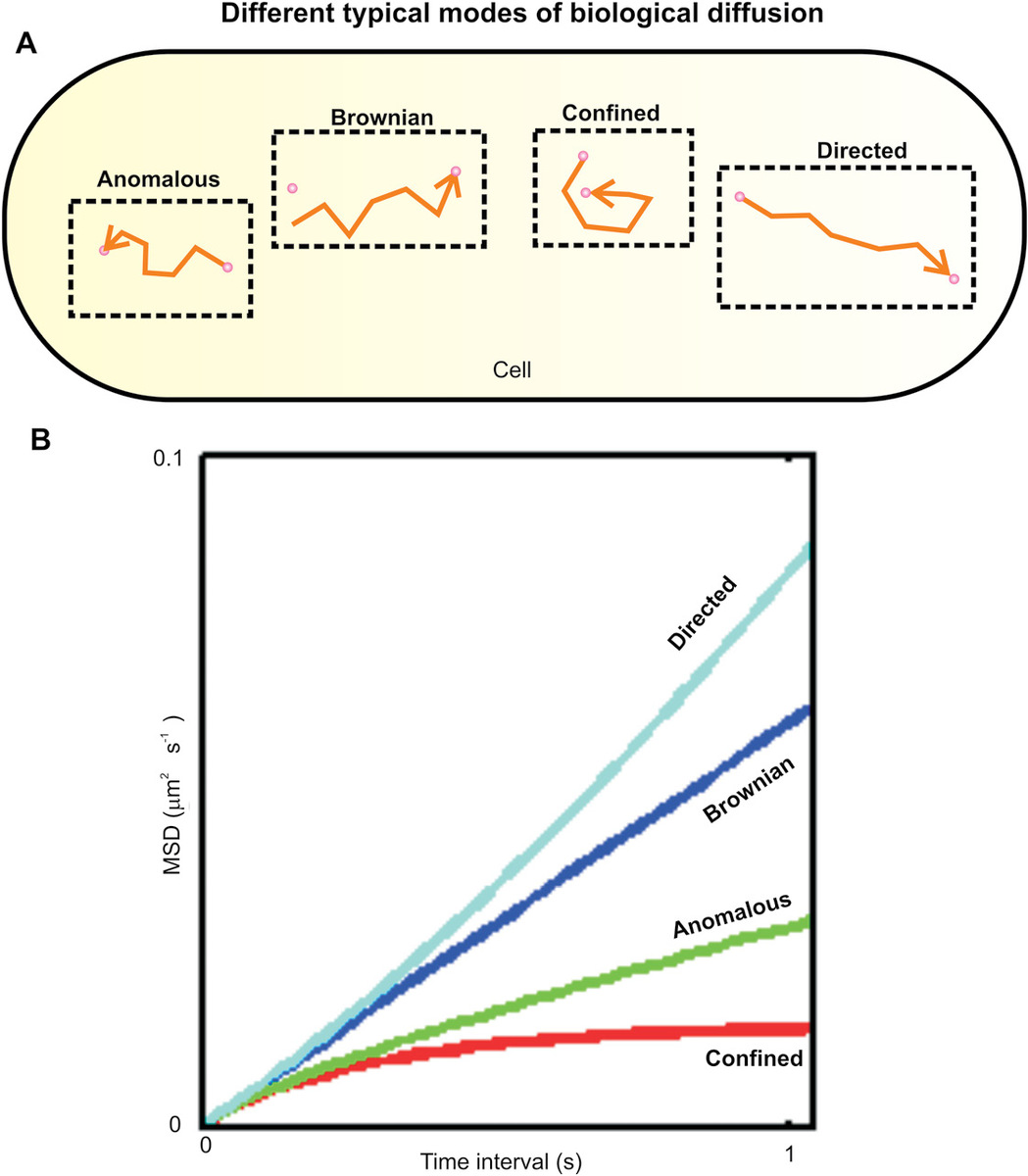
Figure 8.6 Different diffusion modes. (a) Schematic cell inside of which are depicted four different tracks of a particle, which exhibits four different common modes of diffusion or anomalous, Brownian confined and directed. (b) These modes have distinctly different relations on mean square displacement with time interval, such that directed is parabolic, Brownian is linear, confined is asymptotic, and anomalous varies as ~τα, where τ is the time interval and α is the anomalous diffusion coefficient such that 0 < α < 1.
In the case of inhomogeneous fluid environments, for example, the mean square displacement of a particle after time interval τ as ~ τα (see Equation 4.18) where a is the anomalous diffusion coefficient and 0 < α < 1, which depends on factors such as the crowding density of obstacles to diffusion in the fluid environment. Confined diffusion has a typically asymptotic shape with τ.
In practice, however, real experimental tracking data of diffusing particles are intrinsically stochastic in nature and also have additional source of measurement noise, which complicates the problem of inferring the mode of diffusion from the shape of the mean square displacement relation with τ. Some experimental assays involve good sampling of the position of tracked diffusing biological particles. An example of this is a protein labeled with a nanogold particle in an in vitro assay involving a similar viscosity environment using a tissue mimic such as collagen to that found in the living tissue. The position of the nanogold particle can be monitored as a function of time using laser dark-field microscopy (see Chapter 3). The scatter signal from the gold tag does not photobleach, and so they can be tracked for long durations allowing a good proportion of the analytical mean square displacement relation to be sampled thus facilitating inference of the type of underlying diffusion mode.
However, the issue of using such nanogold particles is that they are relatively large (tens of nm diameter, an order of magnitude larger than typical proteins investigated) as a probe and so potentially interfere sterically with the diffusion process, in addition to complications with extending this assay into living cells and tissue due to problems of specific tagging of the right protein and its efficient delivery into cells. A more common approach for live-cell assays is to use fluorescence microscopy, but the primary issue here is that the associated tracks can often be relatively truncated due to photobleaching of the dye tag and/or diffusing beyond the focal plane resulting in tracked particles going out of focus.
Early methods of mean square displacement analysis relied simply on determining a metric for linearity of the fit with respect to time interval, with deviations from this indicative of diffusion modes other than regular Brownian. To overcome issues associated with noise on truncated tracks, however, improved analytical methods now often involve aspects of Bayesian inference.
In words, Bayes’ theorem is simply posterior = (likelihood × prior)/evidence.
The definitions of these terms are as follows, which utilizes statistical nomenclature of the conditional probability “P(A|B)” meaning “the probability of A occurring given that B has occurred.” The joint probability for both events A and B occurring is written as P(A∩B). This can be written as the probability of A occurring given that B has occurred:
(8.93)But similarly, this is the same as the probability of B occurring given that A has occurred:
(8.94)Thus, we can arrive at a more mathematical description of Bayes’ theorem, which is
(8.95)Thus, the P(A) is the prior of A, P(B) is the evidence, P(B|A) is the likelihood for B given A, and P(A|B) is the posterior for A given B (i.e., the probability for this occurring given prior knowledge of the probability distributions of A and B).
Bayes’ theorem provides the basis for Bayesian inference as a method for the statistical testing of different hypotheses, such that P(A|B) is then a specific model/hypothesis. Thus, we can say that
(8.96)P(data|model) is an experimentally observed dataset, P(model) is a prior for the given model, and P(model|data) is the resultant prediction for posterior probability that that model accounts for these data. Thus, the higher the values of P(model|data), the more likely it is that the model is a good one, and so different models can thus be compared with each other and ranked to decide which one is the most sensible to use.
For using Bayesian inference to discriminate between different models of diffusion for single-particle tracking data, we can define the following:
- The likelihood, P(d|w,M), where d represents the spatial tracking data from a given biomolecule and w is some general parameters of a specific diffusion model M. This is the probability distribution of the data for a given parameter from this model.
- The prior, P(w|M). This is the initial probability distribution function to any conditioning by the data; priors represent any initial estimate of the system, such as distribution of the parameters or the expected order of magnitude.
- The posterior, P(w|d,M). This is the distribution of the parameter following the conditioning by the data.
- The evidence, P(d|M). This acts as a normalization factor and is a portable unitless quantity.
One such analytical method that employs this strategy in inferring modes of diffusion from molecular tracking data is called “Bayesian ranking of diffusion” (BARD). This uses two stages in statistical inference: first, parameter inference, and second, model selection. The first stage infers the posterior distributions about each model parameter, which is defined as
(8.97)The second stage is model selection:
(8.98)P(M|d) is a number that is the model posterior, or probability. P(M) is a number that is the model prior (model priors are usually flat, indicating that the initial assumption is that all models are expected equally), P(d|M) is a number that is the model likelihood, and P(d) is a number that is a normalizing factor that accounts for all possible models. This now generates the posterior (i.e., probability) for a specific model. Linking the two stages is the term P(d|M), the model likelihood, which is also the normalization term in the first stage. Comparing calculated normalized P(d|M) values for each independent model then allows each model to be ranked from the finite set of diffusion models tried in terms of the likelihood that it accounts for the observed experimental tracking data (e.g., the mean square displacement vs τ values for a given tracked molecule).
8.4.4 Fluid Transport in Biology
Previously in this book, we discussed several examples of fluid dynamics. The core mathematical model for all fluid dynamics processes is embodied in the Navier–Stokes equation. The Navier–Stokes equation results from Newton’s second law of motion and conservation of mass. In a viscous fluid environment under pressure, the total force at a given position in the fluid is the sum of all external forces, F, and the divergence of the stress tensor σ. For a velocity of magnitude v in a fluid of density, ρ this leads to
(8.99)The left-hand side of this equation is equivalent to the mass multiplied by total acceleration in Newton’s second law. The stress tensor is given by the grad of the velocity multiplied by the viscous drag coefficient minus the fluid pressure, which after rearrangement leads to the traditional form of the Navier–Stokes equation of
(8.100)For many real biological processes involving fluid flow, the result is a complicated system of nonlinear PDEs. Some processes can be legitimately simplified, however, in terms of the mathematical model, for example, treating the fluid motion as an intrinsically 1D problem, in which case the Navier–Stokes equation can be reduced in dimensionality, but often some of the terms in the equation can be neglected, and the problem reduced to a few linear differential equations, and sometimes even just one, which facilitates a purely analytical solution. Many real systems, however, need to be modeled as coupled nonlinear PDEs, which makes an analytical solution difficult or impossible to achieve. These situations are often associated with the generation of fluid turbulence with additional random stochastic features, which are not incorporated into the basic Navier–Stokes equation becoming important in the emergence of large-scale pattern formation in the fluid over longer time scales. These situations are better modeled using Monte Carlo–based discrete computational simulations, in essence similar to the molecular simulation approaches described earlier in this chapter but using the Navier–Stokes equation as the relevant equation of motion instead of simply F = ma.
In terms of simplifying the mathematical complexity of the problem, it is useful to understand the physical origin and meaning of the three terms on the right-hand side of Equation 8.100.
The first of these is −(v·∇)·v. This represents the divergence on the velocity. For example, if fluid flow is directed to converge through a constriction, then the overall flow velocity will increase. Similarly, the overall flow velocity will decrease if fluid flow is divergent in the case of a widening of a flow channel.
The second term is −∇p/ρ. This represents the movement of diffusing molecules with changes to fluid pressure. For example, molecules will be forced away from areas of high-pressure changes, specifically, the tendency to move away from areas of higher pressure. If the local density of molecules is high, then a smaller proportion of molecules will be affected by changes in the local pressure gradient. Similarly, at low density, there is a greater proportion of the molecules that will be affected.
The third term is γ∇2v. This represents the effects of viscosity between neighboring diffusing molecules. For example, in a high viscosity fluid (e.g., the cell membrane), there will be a greater correlation between the motions of neighboring biomolecules than in a low viscosity fluid (e.g., the cell cytoplasm). The fourth term F as discussed is the net sum of all other external forces.
In addition to reducing mathematical descriptions to a 1D problem where appropriate, further simplifications can often involve neglecting the velocity divergence and external force terms, the governing equation of motion can often then be solved relatively easily, for example, in the case of Hagen–Poiseuille flow in a microfluidics channel (see Chapter 7) and also fluid movement involving laminar flow around biological structures that can be modeled acceptably by well-defined geometrical shapes. The advantage here is that well-defined shapes have easily derived analytical formulations for drag coefficients, for example, that of a sphere is manifested in Stokes law (see Chapter 6) or that of a cylinder that models the effects of drag on transmembrane proteins (see Chapter 3), or that of a protein or nucleic acid undergoing gel electrophoresis whose shape can be modeled as an ellipsoid (see Chapter 6). The analysis of molecular combining (see Chapter 6) may also utilize cylindrical shapes as models of biopolymers combed by the surface tension force of a retracting fluid meniscus, though better models involve characterizing the biopolymers as WLC, which is reptating within the confines of a virtual tube and thus treating the viscous drag forces as those on the surface of this tube.
Fluid dynamics analysis is also relevant to swimming organisms. The most valuable parameter to use in terms of determining the type of analytical method to employ to model swimming behavior is the dimensionless Reynolds number Re (see Chapter 6). Previously, we discussed this in the context of allowing us to determine if fluid flow was turbulent or laminar, such that Re values above a rough cutoff of ~2100 (see Chapter 7). The importance for swimming organisms is that there are two broadly distinct regimes of low Reynolds number swimmers and high Reynolds number swimmers.
High Reynolds number hydrodynamics involve in essence relatively large, fast organisms resulting in Re > 1. Conversely, low Reynolds number hydrodynamics involve in essence relatively small, slow organisms resulting in Re < 1. For example, a human swimming in water has a characteristic length scale of ~ 1 m, with a typical speed of ~1 m s−1, indicating an Re of ~106.
Low Reynolds number swimmers are typically microbial, often single-cell organisms. For example, E. coli bacteria have a characteristic length scale of ~1 μm but have a typical swimming speed of a few tens of microns every second. This indicates a Re of ~10−5.
High Reynolds number hydrodynamics are more complicated to analyze since the complete Navier–Stokes equation often needs to be considered. Low Reynolds number hydrodynamics is far simpler. This is because the viscous drag force on the swimming organism is far in excess of the inertial forces. Thus, when a bacterial cell stops actively swimming, then the cell motion, barring random fluid fluctuations, stops. In other words, there is no gliding.
For example, consider the periodic back-and-forth motions of an oar of a rowing boat in water, a case of high Re hydrodynamics. Such motions will propel the boat forward. However, for low Re hydrodynamics, this simple reciprocal motion in water will result in a net swimmer movement of zero. Thus, for bacteria and other microbes, their swimming motion needs to be more complicated. Instead of a back-and-forth, bacteria rotate a helical flagellum to propel themselves, powered by a rotary molecular machine called the flagellar motor, which is embedded in the cell membrane. This acts in effect as a helical propeller.
Bacteria utilize this effect in bacterial chemotaxis that enables them to swim up a chemical nutrient gradient to find source of food. The actual method involves a biased random walk. For example, the small length scale of E. coli bacteria means that they cannot operate a system of different locations of nutrient receptor on their cell surface to decide which direction to swim since there would be insufficient distance between any two receptors to discriminate subtle differences of a nutrient concentration over a ~1 μm length scale. Instead, they operate a system of alternating runs and tumbles in their swimming, such that a run involves a bacterial cell swimming in a straight line and a tumble involving the cell stopping but then undergoing a transient tumbling motion that then randomizes the direction of the cell body prior to another run that will then be in a direction largely uncorrelated with the previous run (i.e., random).
The great biological subtlety of E. coli chemotaxis is that the frequency of tumbling increases in a low nutrient concentration gradient but decreases in a high nutrient concentration gradient using a complicated chemical cascade and adaption system that involves feedback between chemical receptors on the cell membrane and the flagellar motor that power the cell swimming via diffusion-mediated signal transduction of a response regulator protein called CheY through the cell cytoplasm. This means that if there is an absence of food locally, the cell will change its direction more frequently, whereas if food is abundant, the cell will tumble less frequently, ultimately resulting in a biased random walk in the average direction of a nutrient concentration gradient (i.e., in the direction of food). Remarkably, this system does not require traditional gene regulation (see Chapter 7) but relies solely on interactions between a network of several different chemotaxis proteins.
8.5 Advanced In Silico Analysis Tools
Computational analysis of images is of core importance to any imaging technique, but the most basic light microscopy technique. The challenge here is to automate and objectify detection and quantitation. In particular, advances in low-light fluorescence microscopy have allowed single-molecule imaging experiments in living cells across all three domains of life to become commonplace. Many open-source computational software packages are available for image analysis, the most popular of which is ImageJ, which is based on a Java platform and has an extensive back catalog of software modules written by members of the user community. C/C++ is a popular computational language of choice for dedicated computationally efficient image analysis, while the commercial language MATLAB is ideal for the development of new image analysis routines as it benefits from extensive image analysis coding libraries as well as an enthusiastic user community that regularly exchanges ideas and new beta versions of code modules.
Single-molecule live-cell data are typically obtained in a very low signal-to-noise ratio regime often only marginally in excess of 1, in which a combination of detector noise, suboptimal dye photophysics, natural cell autofluorescence, and underlying stochasticity of biomolecules results in noisy datasets for which the underlying true molecular behavior is nontrivial to observe. The problem of faithful signal extraction and analysis in a noise-dominated regime is a “needle in a haystack” challenge, and experiments benefit enormously from a suite of objective, automated, high-throughput analysis tools that detect underlying molecular signatures across a large population of cells and molecules. Analytical computational tools that facilitate this detection comprise methods of robust localization and tracking of single fluorescently labeled molecules, analysis protocols to reliably estimate molecular complex stoichiometry and copy numbers of molecules in individual cells, and methods to objectively render distributions of molecular parameters. Aside from image analysis computational tools, there are also a plethora of bioinformatics computational tools that can assist with determining molecular structures in particular.
8.5.1 Image Processing, Segmentation, and Recognition
The first stage of image processing is generally the eradication of noise. The most common way to achieve this is by applying low-pass filters in the Fourier space of the image, generated from the discrete Fourier transform (DFT), to block higher spatial frequency components characteristic of pixel noise, and then reconstructing a new image using the discrete inverse Fourier transform. The risk here is a reduction in equivalent spatial resolution. Other methods of image denoising operate in real space, for example, using 2D kernel convolution that convolves each pixel in the image with a well-defined 2D kernel function, with the effect of reducing the noise on each pixel by generating a weighted averaging signal output involving it and several pixels surrounding it, though as with Fourier filtering methods a caveat is often a reduction in spatial resolution manifest as increased blurring on the image, though some real space denoising algorithms incorporate components of feature detection in images and so can refine the denoising using an adaptive kernel, that is, to increase the kernel size in relatively featureless regions of an image but decrease it for regions suggesting greater underlying structure.
Several other standard image processing algorithms may also be used in the initial stages of image analysis. These include converting pixel thresholding to convert raw pixel intensity into either 0 or 1 values, such that the resulting image becomes a binary large object (BLOB). A range of different image processing techniques can then be applied to BLOBs. For example, erosion can trim off outer pixels in BLOB hotspots that might be associated with noise, whereas dilation can be used to expand the size of BLOBs to join proximal neighboring BLOBs into a single BLOB, the reason being again that this circumvents the artifactual effects of noise that can often have an effect to make a single foreground object feature in an image that appear to be composed of multiple separate smaller foreground objects.
Light microscopy bright-field images of cells and tissues, even using enhancement methods such as phase contrast or DIC (see Chapter 3), result in diffraction-limited blurring of the cellular boundary and of higher length scale tissue structures. Several image segmentation techniques are available that can determine the precise boundaries of cells and tissue structures. These enable cell bodies and structures to be separately masked out and subjected to further image analysis, in addition to generating vital statistics of cell and tissue structure dimensions. Vital statistics are valuable for single-cell imaging in model bacteria in being used to perform coordinate transformations between the Cartesian plane of the camera detector and the curved surface of a cell, for example, if tracking the diffusion of a membrane protein on the cell’s surface. The simplest and most computationally efficient method involves pixel intensity thresholding that in essence draws a contour line around a cell image corresponding to a preset pixel intensity value, usually interpolated from the raw pixel data. Such methods are fast and reliable if the cell body pixel intensity distribution is homogeneous.
Often cell images are very close to each other to the extent that they are essentially touching, for example, cell-to-cell adhesions in a complex multicellular tissue or recent cell division events in the case of observation on isolated cells. In these instances simple pixel thresholding tools will often fail to segment these proximal cells. Watershed methods can overcome this problem by utilizing “flooding” strategies. Flooding seed points are first determined corresponding roughly to the center of putative cell objects, and the image is flooded with additional intensity added to pixel values radially from these seeds until two juxtaposed flooding wave fronts collide. This collision interface then defines the segmentation boundary between two proximal cells.
The most robust but computationally expensive cell image segmentation methods utilize prior knowledge of what the sizes and shapes of the specific cells under investigation are likely to be. These can involve Bayesian inference tools utilizing prior knowledge from previous imaging studies, and many of these approaches use maximum entropy approaches to generate optimized values for segmentation boundaries. Similarly, maximum a posteriori methods using Bayesian statistics operate by minimizing an objective energy function obtained from the raw image data to determine the most likely position of cell boundaries.
Many molecular structures visualized in biological specimens using high-spatial-resolution imaging techniques such as EM, AFM, and super-resolution light microscopy may exhibit a distribution on their orientation in their image data, for example, due to random orientation of the structure in the specimen itself and/or to random orientation of cells/tissues in the sample with respect to the imaging plane. To facilitate identification of such structures, there are algorithms that can rotate images and compare them with reference sources to compare in computationally efficient ways. This usually involves maximum likelihood methods that generate a pixel-by-pixel cross-correlation function between the candidate-rotated image and the reference source and find solutions that optimize the maximum cross-correlation, equivalent to template matching.
However, the most widely used method to recognize specific shapes and other topological and intensity features of images is principal component analysis (PCA). The general method of PCA enables identification of the principal directions in which the data vary. In essence, the principal components, or normal modes, of a general dataset are equivalent to axes that can be in multidimensional space, parallel to which there is most variation in the data. There can be several principal components depending on the number of independent/orthogonal features of the data. In terms of images, this in effect represents an efficient method of data compression, by reducing the key information parallel to typically just a few tens of principal components that encapsulate just the key features of an image.
In computational terms, the principal components of an image are found from a stack of similar images containing the same features and then calculating the eigenvectors and eigenvalues of the equivalent data covariance matrix for the image stack. An eigenvector that has the largest eigenvalue is equivalent to the direction of the greatest variation, and the eigenvector with the second largest eigenvalue is an orthogonal direction that has the next highest variation, and so forth for higher orders of variation beyond this. These eigenvectors can then be summed to generate a compressed version of any given image such that if more eigenvectors are included, then the compression is lower and the quality of the compressed image is better.
Each image of area i × j pixels may be depicted as a vector in (i × j)2 dimensional hyperspace, which has coordinates that are defined by the pixel intensity values. A stack of such images is thus equivalent to a cloud of points defined by the ends of these vectors in this hyperspace such that images that share similar features will correspond to points in the cloud that are close to each other. A pixel-by-pixel comparison of all images as is the case in maximum likelihood methods is very slow and computationally costly. PCA instead can reduce the number of variables describing the stack imaging data and find a minimum number of variables in the hyperspace, which appear to be uncorrelated, that is, the principal components. Methods involving multivariate statistical analysis (MSA) can be used to identify the principal components in the hyperspace; in essence, these generate an estimate for the covariance matrix from a set of images based on pairwise comparisons of images and calculate the eigenvectors of the covariance matrix.
These eigenvectors are a much smaller subset of the raw data and correspond to regions in the image set of the greatest variation. The images can then be depicted in a compressed form with relatively little loss in information since small variations are in general due to noise as the linear sum of a given set of the identified eigenvectors, referred to as an eigenimage.
PCA is particularly useful in objectively determining different image classes from a given set on the basis of the different combinations of eigenvalues of the associated eigenvectors. These different image classes can often be detected as clusters in m-dimensional space where m is the number of eigenvectors used to represent the key features of the image set. Several clustering algorithms are available to detect these, a common one being k-means that links points in m-dimensional space into clusters on the basis of being within a threshold nearest-neighbor separation distance. Such methods have been used, for example, to recognize different image classes in EM and cryo-EM images in particular (see Chapter 5) for molecular complexes trapped during the sample preparation process in different metastable conformational states. In thus being able to build up different image classes from a population of several images, averaging can be performed separately within each image class to generate often exquisite detail of molecular machines in different states. From simple Poisson sampling statistics, averaging across n such images in a given class reduces the noise on the averaged imaged by a factor of ~√n. By stitching such averages from different image classes together, a movie can often be made to suggest actual dynamic movements involved in molecular machines. This was most famously performed for the stepping motion of the muscle protein myosin on F-actin filaments.
Algorithms involving the wavelet transform (WT) are being increasingly developed to tackle problems of denoising, image segmentation, and recognition. For the latter, WT is a complementary technique to PCA. In essence, WT provides an alternative to the DFT but decomposes an image into two separate spatial frequency components (high and low). These two components can then be combined to the given four separate resulting image outputs. The distribution of pixel intensities in each of these four WT output images represents a compressed signature of the raw image data. Filtering can be performed by blocking different regions of these outputs and then reconstructing a new image using the inverse WT in the same way as filtering of the DFT image output. Similarly various biological features can be identified such as cellular boundaries (which can be used for image segmentation) and in general image class recognition. PCA is ultimately more versatile in that the user has the choice to vary the number of eigenvectors to represent a set of images depending on what image features are to be detected; however, WT recognition methods are generally computationally more efficient and faster (e.g., “smart” missile technology for military applications often utilize WT methods). A useful compromise can often be made by generating hybrid WT/PCA methods.
8.5.2 Particle Tracking and Molecular Stoichiometry Tools
As discussed previously, localization microscopy methods can estimate the position of the intensity centroid of a point spread function image (typically a fluorescent spot of a few hundred nanometers of width) from a single dye molecule imaged using diffraction-limited optics to pinpoint the location of the dye to a precision, which is one to two orders of magnitude smaller than the standard optical resolution limit (see Chapter 4). The way this is achieved in practice computationally is first to identify the candidate spots automatically using basic image processing as the previously to determine suitable hotspots in each image and second to define a small region of interest around each candidate spot, typically a square of 10–20 pixels edge length. The pixel intensity values in this region can then be fitted by an appropriate function, usually a 2D Gaussian as an approximation to the center of the Airy ring diffraction pattern, generating not only an estimate of the intensity centroid but also the total brightness I(t) of the spot at a time t and of the intensity of the background in image in the immediate vicinity of each spot.
Spots in subsequent image frames may be linked provided that they satisfy certain criteria of being within a certain range of size and brightness of a given spot in a previous image frame and that their intensity centroids are separated by less than a preset threshold often set close to the optical resolution limit. If spots in two or more consecutive image frames satisfy these criteria, then they can be linked computationally to form a particle track.
The spatial variation of tracks with respect to time can be analyzed to generate diffusion properties as described earlier. But also the spot brightness values can be used to determine how many dye molecules are present in any given spot. This is important because many molecular complexes in biological systems have a modular architecture, meaning that they consist of multiple repeats of the same basic subunits. Thus, by measuring spot brightness, we can quantify the molecular stoichiometry subunits, depending upon what component a given dye molecule is labeling.
As a fluorescent-labeled sample is illuminated, it will undergo stochastic photobleaching. For simple photobleaching processes, the “on” time of a single dye molecule has an exponential probability distribution with a mean on time of tb. This means that a molecular complex consisting of several such dye tags will photobleach as a function of time as ~exp(−t/tb) assuming no cooperative effects between the dye tags, such as quenching. Thus, each track I(t) detected from the image data can be fitted using the following function:
(8.108)which can be compared with Equation 3.32 and used to determine the initial intensity I0 at which all dye molecules are putatively photoactive. If ID is the intensity of a single dye molecule under the same imaging conditions, then the stoichiometry S is estimated as
(8.109)The challenge is often to estimate an accurate value for ID. For purely in vitro assays, individual dye molecule can be chemically immobilized onto glass microscope coverslip surfaces to quantify their mean brightness from a population. However, inside living cells, the physical and chemical environment can often affect the brightness significantly. For example, laser excitation light can be scattered inside a cellular structure, but also the pH and the presence of ions such as chloride Cl−, in particular, can affect the brightness of fluorescent proteins in particular (see Chapter 3).
Thus, it is important for in vivo fluorescence imaging to determine ID in the same native cellular context. One way to achieve this is to extract the characteristic periodicity in intensity of each track, since steplike events occur in the intensity traces of tracks due to integer multiples of dye molecule photobleaching within a single sampling time window. Fourier spectral methods are ideal for extracting the underlying periodicity of these step events and thus estimating ID (Figure 8.8).
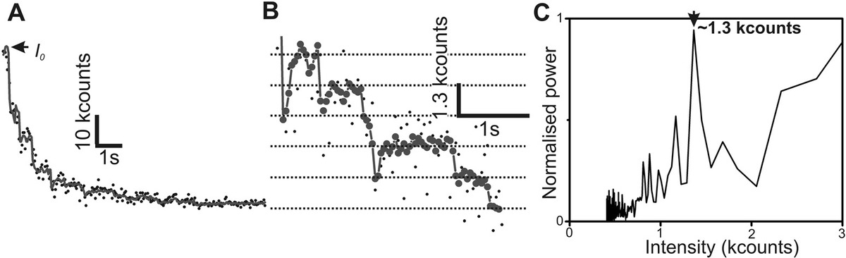
Figure 8.8 Measuring stoichiometry using stepwise photobleaching of fluorophores. (a) Example of a photobleach trace for a protein component of a bacterial flagellar motor called FliM labeled with the yellow fluorescent protein YPet, raw data (dots), and filtered data (line) shown, initial intensity indicated (arrow), with (b) a zoom-in of trace and (c) power spectrum of the pairwise difference distribution of these photobleaching data, indicating a brightness of a single YPet molecule of ~1.3 kcounts on the camera detector used on the microscope.
Often molecular complexes will exhibit an underlying distribution of stoichiometry values. Traditional histogram methods of rendering this distribution for subsequent analysis are prone to subjectivity errors since they depend on the precise position of histogram bin edges and of the number of bins used to pool the stoichiometry data. A more objective and robust method involves kernel density estimation (KDE). This is a 1D convolution of the stoichiometry data using a Gaussian kernel whose integrated area is exactly 1 (i.e., representing a single point), and the width is a measure of the experimental error of the data measurement. This avoids the risks in particular of using too many histogram bins that suggest more multimodality in a distribution than really exists or too few bins that may suggest no multimodality when, in fact, there may well be some (Figure 8.9).
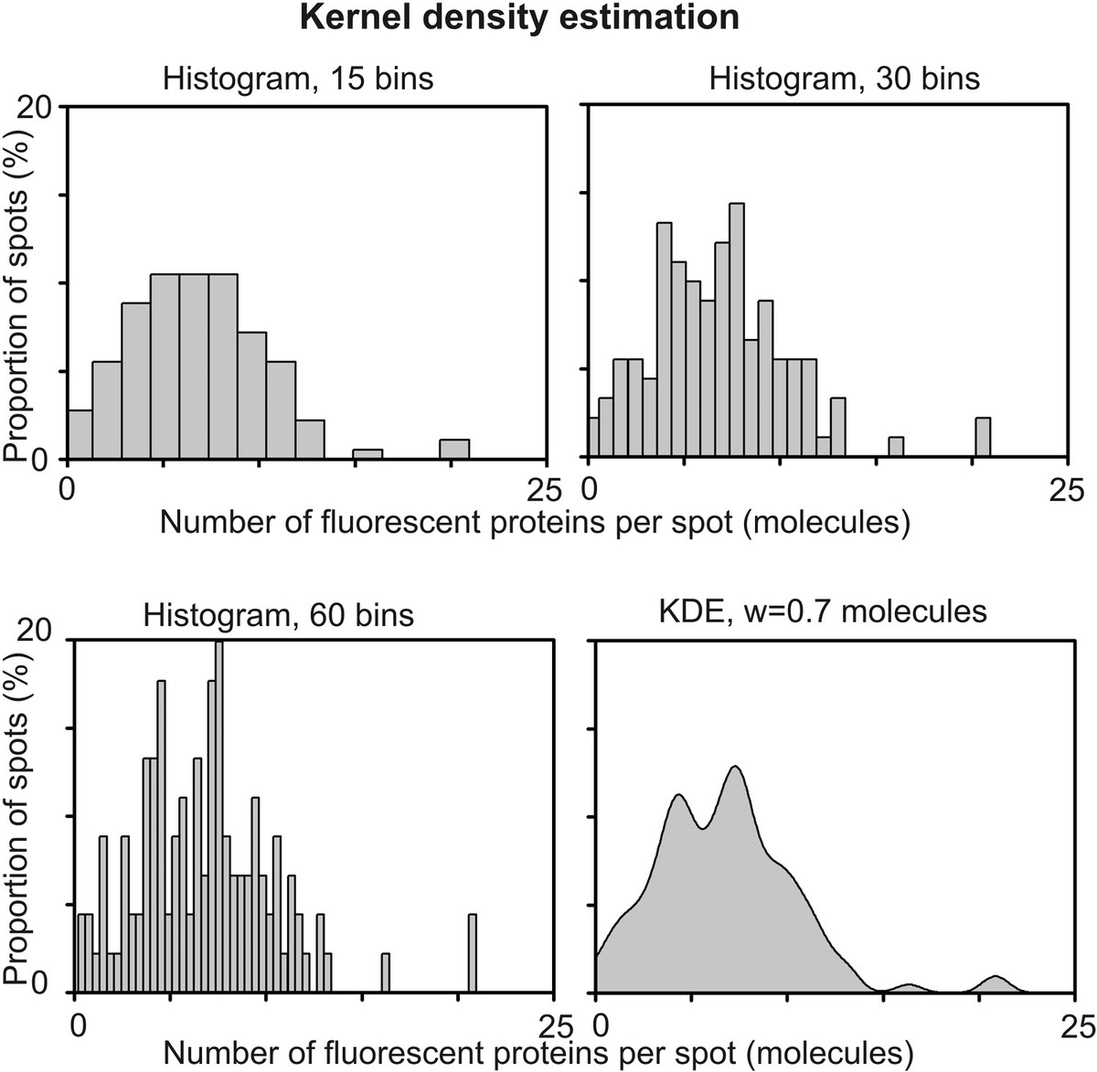
Figure 8.9 Using kernel density estimation to objectify stoichiometry distributions. Too few histogram bins can mask underlying multimodality in a distribution, whereas too many can give the impression of more multimodality than really exists. A kernel density estimation (here of width w = 0.7 molecules, equivalent to the measurement error in this case) generates an objective distribution.
Sometimes there will be periodicity in the observed experimental stoichiometry distributions of molecular complexes across a population, for example, due to modality of whole molecular complexes themselves in tracked spots. Such periodicity can again be determined using basic Fourier spectral methods.
8.5.3 Colocalization Analysis for Determining Molecular Interactions in Images
Experiments to monitor molecular interactions have been revolutionized by multicolor fluorescence microscopy techniques (see Chapter 3). These enable one to monitor two or more different molecular components in a live biological sample labeled with different color dye that can be detected via separate color channels. The question then is to determine whether or not two such components really are interacting, in which case they will be colocalized in space at the same time. However, the situation is complicated by the optical resolution limit being several hundred nanometers, which is two orders of magnitude larger than the length scale over which molecular interactions occur.
The extent of colocalization of two given spots in separate color channels can best be determined computationally by constructing an overlap integral based on the fit outputs from the localization tracking microscopy. Each candidate spot is first fitted using a 2D Gaussian as before, and these functions are then normalized to give two Gaussian probability distribution functions g1 and g2, centered around (x1, y1) with width σ1 and around (x2, y2) with width σ2, respectively, and defined as
(8.110)Their unnormalized overlap can be calculated from the integral of their product:
(8.111)where
- Δr is the distance between the centers of the Gaussians on the xy image plane
- C is a normalization constant equal to the maximum overlap possible for two perfectly overlapped spots so that
The normalized overlap integral, v, for a pair of spots of known positions and widths, is then
(8.114)The value of this overlap integral can then be used as a robust and objective measure for the extent of colocalization. For example, for “optical resolution colocalization,” which is the same as the Rayleigh criterion (see Chapter 3), values of ~0.2 or more would be indicative of putative colocalization.
One issue with this approach, however, is that if the concentration of one or the both of the molecules under investigation are relatively high (note, biologists often refer to such cells as having high copy numbers for a given molecule, meaning the average number of a that given molecule per cell), then there is an increasing probability that the molecules may appear to be colocalized simply by chance, but are in fact not interacting. One can argue that if two such molecules are not interacting, then after a short time their associated fluorescent spots will appear more apart from each other; however, in practice, the diffusion time scale may often be comparable to the photobleaching time scale, meaning that these chance colocalized dye molecules may photobleach before they can be detected as moving apart from each other.
It is useful to predict the probability of such chance colocalization events. Using nearest-neighbor analysis for a random distribution of particles on a 2D surface, we can determine the probability p(r) dr that the distance from one fluorescent spot in the cell to another of the same type is between r and r + dr. This analysis results in effect in a value of the limiting concentration for detecting distinct spots (see Chapter 4) when averaged over a whole cell and depends upon certain geometrical constraints (e.g., whether a molecule is located in the three spatial dimension cell volume or is confined to two dimensions as in the cell membrane or one dimension as for translocation of molecular motors on a filament). As a rough guide, this is equivalent to ~1017 fluorescent spots per liter for the case of molecules inside the cell volume, which corresponds to a molar concentration of ~100 nM. For interested students, an elegant mathematical treatment for modeling this nearest-neighbor distance was first formulated by one of the great mathematicians of modern times (Chandrasekhar, 1943) for a similar imaging problem but involving astrophysical observations of stars and planets.
For example, consider the 2D case of fluorescent spots located in the cell membrane. The probability p(r)dr must be equal to the probability that there are zero such fluorescent spots particles in the range 0−r, multiplied by the probability that a single spot exists in the annulus zone between r and r + dr. Thus,
(8.115)where n is the number of fluorescent spots per unit area in the patch of cell membrane observed in the focal plane using fluorescence microscopy. Solving this equation and using the fact that this indicates that p → 2πrn in the limit r → 0, we obtain:
(8.116)Thus, the probability p1(w) that the nearest-neighbor spot separation is greater than a distance w is
(8.117)The effective number density per unit area, n, at the focal plane is given by the number of spots Nmem observed in the cell membrane on average for a typical single image frame divided by the portion, ΔA, of the cell membrane imaged in focus that can be calculated from a knowledge of the depth of field and the geometry of the cell surface (see Chapter 3). (Note in the case of dual-color imaging, Nmem is the total summed mean number of spots for both color channels.)
The probability that a nearest-neighbor spot will be a distance less than w away is given by 1 − p1(w) = 1 − exp(−πw2Nmem/A). If w is then set to be the optical resolution limit (~200–300 nm), then an estimate for 1 − p1(w) is obtained. Considering the different permutations of colocalization or not between two spots from different color channels indicates that the probability of chance colocalization pchance of two different color spots is two-thirds of that value:
(8.118)It is essential to carry out this type of analysis in order to determine whether the putative colocalization observed from experimental data is likely due to real molecular interactions or just to expectations from chance.
8.5.4 Convolution Modeling to Estimate Protein Copy Numbers in Cells
Fluorescence images of most cells containing which specific mobile molecule has been fluorescently labeled inevitably are composed of a distinct spot component, that is, distinct fluorescent spots that have been detected and tracked and a diffusive pool component. The latter may be composed of fluorescent spots that have not been detected by automated code, for example, because the local nearest-neighbor separation distance was less than the optical resolution, but also may often comprise dimmer, faster moving spots that are individual subunits of the molecular complexes that are brighter and diffuse more slowly and thus are more likely to be detected in tracking analysis.
Convolution models can quantify this diffusive pool component on a cell-by-cell basis. This is valuable since it enables estimates to be made of the total number of fluorescently labeled molecules in a given cell if combined with information from the number and stoichiometry of tracked distinct fluorescent spots. In other words, the distribution of copy number for that molecule across a population of cell can be quantified, which is useful in its own right, but which can also be utilized to develop models of gene expression regulation.
The diffusive pool fluorescence can be modeled as a 3D convolution integral of the normalized PSF, P, of the imaging system, over the whole cell. Every pixel on the camera detector of the fluorescence microscope has a physical area ΔA with equivalent area dA in the conjugate image plane of the sample mapped in the focal plane of the microscope:
(8.119)where M is the total magnification between the camera and the sample. The measured intensity, I′, in a conjugate pixel area dA is the summation of the foreground intensity I due to dye molecules plus any native autofluorescence (Ia) plus detector noise (Id). I is the summation of the contributions from all of the nonautofluorescence fluorophores in the whole of the cell:
(8.120)where
- Is is the integrated intensity of a single dye (i.e., its brightness)
- ρ is the dye density in units of molecules per voxel (i.e., one pixel volume unit)
- E is a function that represents the change in the laser profile excitation intensity over a cell
In a uniform excitation field, E = 1, for example, as approximated in wide-field illumination since cells are an order of magnitude smaller than the typical Gaussian sigma width of the excitation field at the sample. For narrow-field microscopy, the excitation intensity is uniform with height z but has a 2D Gaussian profile in the lateral xy plane parallel to the focal plane. Assuming a nonsaturating regime for fluorescent photon emission of a given dye, the brightness of that dye, assuming simple single-photon excitation, is proportional to the local excitation intensity; thus,
(8.121)where σxy is the Gaussian width of the laser excitation field in the focal plane (typically a few microns). In Slimfield, there is an extra small z dependence also with Gaussian sigma width, which is ~2.5 that of the σxy value (see Chapter 3). Thus,
(8.122)Defining C(x0,y0,z0) as a numerical convolution integral and also comprising the Gaussian excitation field dependence over a cell, and assuming the time-averaged dye density is uniform in space, we can calculate the dye density, in the case of a simple single internal cellular compartment, as
(8.123)The mean value of the total background noise (Ia + Id) can usually be calculated from parental cells that do not contain any foreign fluorescent dye tags. In a more general case of several different internal cellular compartments, this model can be extended:
(8.124)where ρj is the mean concentration of the jth compartment, which can be estimated from this equation by least squares analysis. An important feature of this model is that each separate compartment does not necessarily have to be modeled by a simple geometrical shape (such as a sphere) but can be any enclosed 3D volume provided its boundaries are well-defined to allow numerical integration.
Distributions of copy numbers can be rendered using objective KDE analysis similar to that used for stoichiometry estimation in distinct fluorescent spots. The number of protein molecules per cell has a typically asymmetrical distribution that could be fitted well using a random telegraph model for gene expression that results in a gamma probability distribution p(x) that has similarities to a Gaussian distribution but possesses an elongated tail region:
(8.125)where Γ(a) is a gamma function with parameters a and b determined from the two moments of the gamma distribution by its mean value m and standard deviation, such that a = m2/σ2 and b = σ2/m.
8.5.5 Bioinformatics Tools
Several valuable computational bioinformatics tools are available, many developed by the academic community and open source, which can be used to investigate protein structures and nucleotide sequences of nucleic acid, for example, to probe for the appearance of the same sequence repeat in different sets of proteins or to predict secondary structures from the primary sequences. These algorithms operate on the basis that amino acids can be pooled in different classes according to their physical and chemical properties (see Chapter 2). Thus, to some extent, there is interchangeability between amino acids within the same class such that an ultimate secondary, tertiary, and quaternary structure may be similar. These tools are also trained using predetermined structural data from EM, NMR, and x-ray diffraction methods (see Chapter 5), enabling likely structural motifs to be identified from their raw sequence data alone. The most common algorithm used is the basic alignment search tool (BLAST).
Homology modeling (also known as comparative modeling) is a bioinformatics tool for determining atomic-level resolution molecular structures. It is most commonly performed on proteins operating by interpolating a sequence, usually the primary structure of amino acid residues, of a molecule with unknown structure to generate an estimate for that structure, known as the target, onto a similar structure of a molecule known as the template, which is of the same or similar structural family. The algorithms have similarity to those used in BLAST.
Protein structures are far more conserved than protein sequences among such homologs perhaps for reasons of convergent evolution; similar tertiary structures evolve from different primary structures which imparts a selective advantage on that organism (but note that primary sequences with less than 20% sequence identity often belong to different structural families). Protein structures are in general more conserved than nucleic acid structures. Alignment in the homology fits is better in regions of distinct secondary structures being forms (e.g., α-helices, β-sheets; see Chapter 2) and similarly is poorer in random coil primary structure regions.
8.5.6 Step Detection
An increasingly important computational tool is the automation of the detection of steps in noisy data. This is especially valuable for data output from experimental single-molecule biophysics techniques. The effective signal-to-noise ratio is often small and so the distinction between real signal and noise is often challenging to make and needs to be objectified. Also, single-molecule events are implicitly stochastic and depend upon the underlying probability distribution for their occurrence that can often be far from simple. Thus, it is important to acquire significant volumes of signal data, and therefore, an automated method to extract real signal events is useful. The transition times between different molecular states are often short compared to sampling time intervals such that a “signal” is often manifested as a steplike change as a function of time in some physical output parameter, for example, nanometer-level steps in rapid unfolding domain events of a protein stretched under force (see Chapter 6), picoampere level steps in current in the rapid opening and closing of an ion channel in a cell membrane (see Chapter 5), and rapid steps in brightness due to photobleaching events of single dye molecules (see the previous text).
One of the simplest and robust ways to detect steps in a noisy, extended time series is to apply a running window filter that preserves the sharpness and position of a step edge. A popular method uses a simple median filter, which runs a window of number n consecutive data points in a time series on the data such that the running output is the median from data points included in the window. A common method to deal with a problem of potentially having 2n fewer data points in the output than in the raw data is to reflect the first and last n data points to the beginning and end of the time series. Another method uses the Chung–Kennedy filter. The Chung–Kennedy filter consists of two adjacent windows of size n run across the data such that the output switches between the two windows in being the mean value from the window that has the smallest variance (Figure 8.10). The logic here is that if one edge encapsulates a step event, then the variance in that window is likely to be higher.
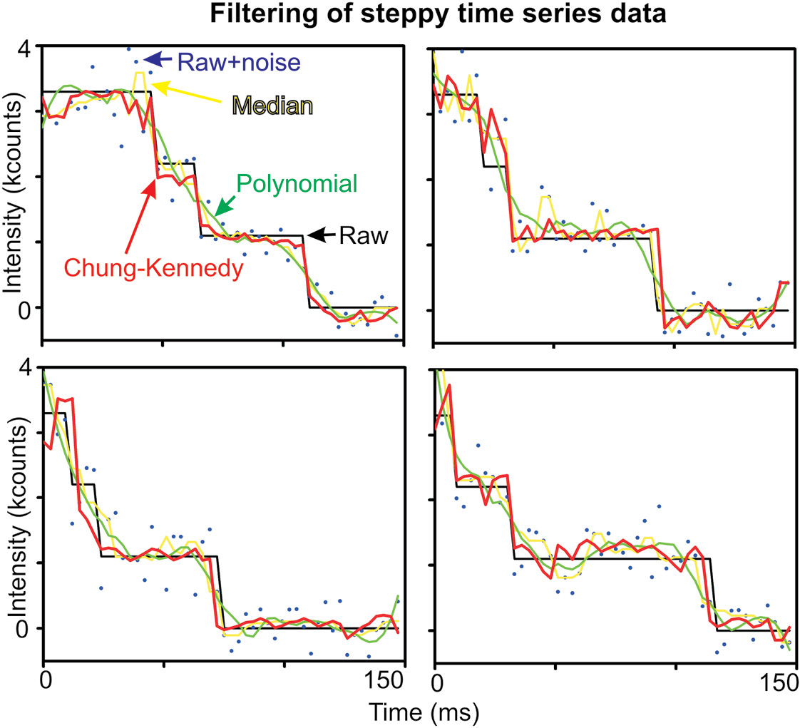
Figure 8.10 Filtering steppy data. Four examples of simulated photobleach steps for a tetramer complex. Raw, noise-free simulated data are shown (line), with noise added (dots), applied with either Chung–Kennedy, median, or a polynomial fit filter. The latter is not edge preserving and so blurs out the distinct step edges.
Both median and Chung–Kennedy filters converge on the same expected value, though the sample variance on the expected value of a mean distribution (i.e., the square of the standard error of the mean) is actually marginally smaller than that of a median distribution; the variance on the expected value from a sampled median distribution is σ2π/2n, which compares with the sample mean of σ2/n (students seeking solace in high-level statistical theory should see Mood et al., 1974), so the error on the expected median value will be larger by a factor of ~√(π/2) or ~25%. There is therefore an advantage in using the Chung–Kennedy filter. Both filters require that the size of n is less than the typical interval between step events; otherwise, the window encapsulates multiple steps and generates nonsensible outputs, so it requires ideally some prior knowledge of likely stepping rates. These edge-preserving filters improve the signal-to-noise ratio for noisy time series by a factor of ~√n. The decision of whether a putative step event is real or not can be made on the basis of the probability of the observed size of the putative step in light of the underlying noise. One way to achieve this is to perform a Student’s t-test to examine if the mean values of the data, <x>, on either side over a window of size n of the putative step are consistent being sampled from the same underlying distribution in light of the variance values on either side of the putative step, σ2, by estimating the equivalent t statistic:
(8.126)This can then be converted into an equivalent probability, and thus the step rejected if, at some preset probability confidence limit, it is consistent with the pre- and post-means being sampled from the same distribution. Improved methods of step detection involve incorporating model-dependent features into step acceptance, for example, involving Bayesian inference. The Fourier spectral methods discussed earlier for determining the brightness of a single dye molecule on a photobleach time series improve the robustness of the step size estimate compared with direct step detection methods in real space, since they utilize all of the information included in the whole time series, but sacrifice information as to the precise time at which any individual step event occurs. These Fourier spectral methods can also be used for determining the step size of the translocation of molecular machines on tracks, for example, using optical tweezer methods (see Chapter 6), and in fact were originally utilized for such purposes.
8.6 Rigid-Body and Semirigid-Body Biomechanics
Rigid-body biomechanics is concerned with applying methods of classical mechanics to biological systems. These can involve both continuum and discrete mathematical approaches. Biomechanics analysis crosses multiple length scales from the level of whole animals through to tissues, cells, subcellular structures, and molecules. Semirigid-body biomechanics encapsulates similar themes, but with the inclusion of finite compliance in the mechanical components of the system.
8.6.1 Animal Locomotion
At the high end of the length scale, this includes analysis of whole animal locomotion, be it on land, in sea, or in air. Here, the actions of muscles in moving bones are typically modeled as levers on pivots with the addition of simple linear springs (to model the action of muscles at key locations) and dampers (to model the action of friction). Several methods using these approaches for understanding human locomotion have been developed to assist in understanding of human diseases, but also much work in this area has been catalyzed by the computer video-gaming industry to develop realistic models of human motion.
Comparative biomechanics is the application of biomechanics to nonhuman animals, often used to gain insights into human biomechanics in physical anthropology or to simply study these animals as an end in itself. Animal locomotion includes behaviors such as running/jumping, swimming, and flying, all activities requiring an external energy to accelerate the animal’s inertial mass and to oppose various combinations of opposing forces including gravity and friction. An emergent area of biophysical engineering research that utilizes the results of human models of biomechanics, in particular, is in developing artificial biological materials or biomimetics (see Chapter 9). This crosses over into the field of biotribology, which is the study of friction/wear, lubrication, and contact mechanics in biological systems, particularly in large joints in the human body. For example, joint implants in knees and hips rub against each other during normal human locomotion, and all lubricated by naturally produced synovial fluid, and biotribology analysis can be useful in modeling candidate artificial joint designs and/or engineered cartilage replacement material that can mimic the shock-absorbing properties in the joints of natural cartilage that has been eroded/hardened through disease/calcification effects.
8.6.2 Plant Biomechanics
Plant biomechanics is also an emerging area of research. The biological structures in plants that generate internal forces and withstand external forces are ostensibly fundamentally different from those in animals. For example, there are no plant muscles as such and no equivalent nervous system to enervate these nonexistent muscles anyway. However, there are similarities in the network of filament-based systems in plant cells. These are more based on the fibrous polysaccharide cellulose but have analogies to the cytoskeletal network of animal cells (see Chapter 2).
Also, although there is no established nervous system to control internal forces, there are methods of chemical- and mechanical-based signal transduction to enable complex regulation of plant forces. In addition, at a molecular level, there are several molecular motors in plants that act along similar lines to those in animal cells (see in the following text). Plant root mechanics is also a particularly emergent area of research in terms of advanced biophysical techniques, for example, using light-sheet microscopy to explore the time-resolved features of root development (see Chapter 4). In terms of analytical models, much of these have been more of the level of computational FEA (see in the following text).
8.6.3 Tissue and Cellular Biomechanics
In terms of computational biomechanics approaches, the focus has remained on the length scale of tissues and cells. For tissue-level simulations, these involve coarse-graining the tissue into cellular units, which each obeys relatively simple mechanical rules, and treating these as elements in a FEA. Typically, the mechanical properties of each cell are modeled as single scaler parameters such as stiffness and damping factor, assumed to act homogeneously across the extent of the cell. Cell–cell boundaries are allowed to be dynamic in the model, within certain size and shape constraints.
An example of this is the cancer, heart, and soft tissue environment (Chaste) simulation toolkit developed primarily by research teams in the University of Oxford. Chaste is aimed at multiple length-scale tissue simulations, optimized to cover a range of real biomechanical tissue-level processes as well as implementing effects of electrophysiology feedback in, for example, regulating the behavior of heart muscle contraction. The simulation packages tissue- and cell-level electrophysiology, discrete tissue modeling, and soft tissue modeling. A specific emphasis of Chaste tools includes continuum modeling of cardiac electrophysiology and of cell populations, in addition to tissue homeostasis and cancer formation.
The electrical properties of the heart muscle can be modeled by a set of coupled PDEs that represents the tissue as two distinct continua either inside the cells or outside, which are interfaced via the cell membrane, which can be represented through a set of complex, nonlinear ODEs that describe transmembrane ionic current (see Chapter 6). Under certain conditions, the effect of the extracellular environment can be neglected and the model reduced to a single PDE. Simulation time scales of 10–100 ms relevant to electrical excitation of heart muscle takes typically a few tens of minutes of a computation time on a typical 32 CPU core supercomputer. Cell-population-based simulations have focused to date on the time-resolved mechanisms of bowel cancers. These include realistic features to the geometry of the surface inside the bowel, for example, specialized crypt regions.
Chaste and other biomechanical simulation models also operate at smaller length scale effects of single cells and subcellular structures and include both deterministic and stochastic models of varying degrees of complexity, for example, incorporating the transport of nutrient and signaling molecules. Each cell can be coarse-grained into a reduced number of components, which appear to have largely independent mechanical properties. For example, the nucleus can be modeled as having a distinct stiffness compared to the cytoplasm. Similarly, the cell membrane and coupled cytoskeleton. Refinements to these models include tensor approximations to stiffness values (i.e., implementing a directional dependence on the stiffness parameters).
An interesting analytical approach for modeling the dynamic localization of cells in developing tissues is to apply arguments from foam physics. This has been applied using numerical simulations to the data from complex experimental tissue systems, such as growth regulation of the wings of the fruit fly and fin regeneration in zebrafish. These systems are good models since they have been characterized extensively through genetics and biochemical techniques, and thus many of the key molecular components are well known. However, standard biochemical and genetics signal regulation do not explain the observed level of biological regulation that results in the ultimate patterning of cells in these tissues. What does show promise, however, is to use mechanical modeling, which in essence treats the juxtaposed cells as bubbles in a tightly packed foam.
The key point here is that the geometry of bubbles in foam has many similarities with those of cells in developing tissues, with examples including both ordered and disordered states, but also in the similarities between the topology, size, and shape of foam bubbles compared to tissue cells. A valuable model for the nearest-neighbor interactions between foam bubbles is the 2D granocentric model (see Miklius and Hilgenfelt, 2012); this is a packing model based purely on trigonometric arguments in which the mean free space around any particle (the problem applied to the packing of grain, hence the name) in the system is minimized. Here, the optimum packing density, even with a distribution of different cell sizes, results in each cell in a 2D array having a mean of six neighbors (see Figure 8.11a). The contact angle Φ between any two tightly packed cells can be calculated from trigonometry (in reference to Figure 8.11a) as
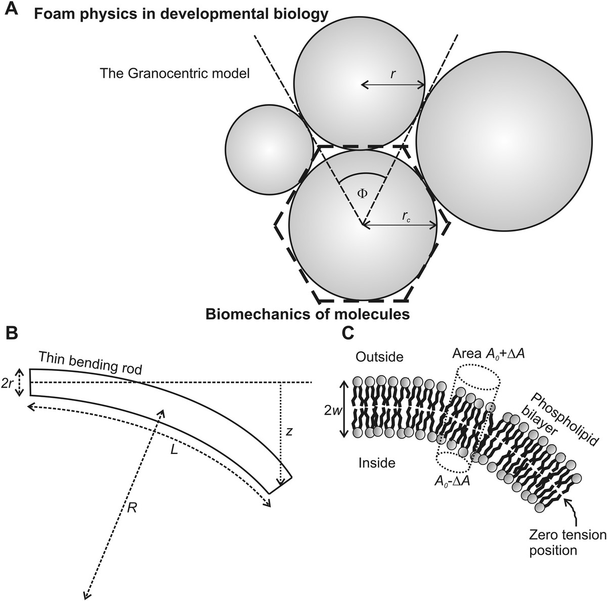
Figure 8.11 Modeling mechanics of cells and molecules. (a) The 2D granocentric model of foam physics—cells are equivalent to the bubbles in the foam, and the contact angle Φ can be calculated using trigonometry from knowledge of the touching cell radii. The mean number of neighbors of a cell is six, as if each cell is an equivalent hexagon (dashed lines). (b) Schematic of bending of a stiff molecular rod. (c) Schematic of bending of a phospholipid bilayer.
Minimizing the free space around cells minimizes the distance to diffusion for chemical signals, maximizes the mechanical efficiency in mechanical signal transduction, and results in a maximally strong tissue. Hence there are logical reasons for cells in many tissues at least to pack in this way.
8.6.4 Molecular Biomechanics
Molecular biomechanics analysis at one level has already been discussed previously in this chapter of biopolymer modeling, which can characterize the relation between molecular force and end-to-end extension using a combination of entropic spring approximations with improvement to correct for excluded volumes and forces of enthalpic origin. In the limit of very stiff biomolecule or filaments, a rodlike approximation, in essence Hooke’s law, is valid, but including also torsional effects such as in the bending cantilever approximation (see Chapter 6). In the case of a stiff, narrow rod of length L and small cross-sectional area dA, if z is a small deflection normal to the rod axis (Figure 8.11b), and we assume that strain therefore varies linearly across the rod, then
(8.128)where R is the radius of curvature of the bent rod. We can then use Hooke’s law and integrate the elastic energy density (Y/2)(ΔL/L)2 over the total volume of the rod, where Y is the Young’s modulus of the rod material, to calculate the total bending energy Ebend:
(8.129)where B is the bending modulus given by YI where I is the moment of inertia. For example, for a cylindrical rod of cross-sectional radius r, I = πr4/4.
An active area of biophysical modeling also involves the mechanics of phospholipid bilayer membranes (Figure 8.11c). Fluctuations in the local curvature of a phospholipid bilayer result in changes to the free energy of the system. The free energy cost ΔG of bilayer area fluctuations ΔA can be approximated from a Taylor expansion centered around the equilibrium state of zero tension in the bilayer equivalent to area A = A0. The first nonzero term in the Taylor expansion is the second-order term:
(8.130)A mechanical parameter called the “area compressibility modulus” of the bilayer, κA, is defined as
(8.131)Thus, the free energy per unit area, Δg, is given by
(8.132)This is useful, since we can model the free energy changes in expanding and contracting a spherical lipid vesicle (e.g., an approximation to a cell). If we say that the area on the outside of a bilayer per phospholipid polar head group (see Chapter 2) is A0 + ΔA and that on the inside of the bilayer is A0 − ΔA since the molecular packing density is greater on the inside than on the outside (see Figure 8.11b), then Δg is equivalent to the free energy change per phospholipid molecule. The total area S of a spherical vesicle of radius R is 4πR2; thus
(8.133)Therefore, the free energy per unit area is given by
(8.134)Equating ΔR with the membrane thickness 2w therefore indicates that the bending free energy cost of establishing this spherical bilayer for a membrane patch area A0 is
(8.135)In other words, there is no direct dependence on the vesicle radius. In practice this can be a few hundred kBT for a lipid vesicle. However, Equation 8.132 implies that relatively large changes to the packing density of phospholipid molecules have a small free energy cost (~kBT or less). This is consistent with phospholipid bilayers being relatively fluid structures.
FEA can also be applied at macromolecular length scales, for example, to model the effects of mesh network of cytoskeletal filaments under the cell membrane and how these respond to external mechanical perturbations. This level of mesoscale modeling can also be applied to the bending motions of heterogeneous semi-stiff filaments such as those found in cilia, which enable certain cells such as sperm to swim and which can cause fluid flow around cells in tissues.
8.7 Summary Points
- Molecular simulations use Newton’s second law of motion with varying degrees of approximations of atomic energy potentials to predict the motions of atoms as a function of time over a scale from hundreds of picoseconds for ab initio QM simulations to tens of nanoseconds for classical MD and tens of microseconds for CG approaches.
- Water is very important in molecular simulations and may be approximated as an explicit solvent, which is very accurate but computationally expensive, or as an implicit solvent that does not simulate details of individual models but enables longer time scales to be simulated for the same computational effort.
- The mechanics of biopolymers can be modeled using pure entropic forces, with improved modeling incorporating additional effects of enthalpic forces and excluded volumes.
- Reaction–diffusion and Navier–Stokes analysis can often be reduced in complexity for modeling important biological processes to generate tractable models, for example, for characterizing molecular motor translocation of tracks, pattern formation in cell and developmental biology, and the fluid flow around biological particles.
- Bayesian inference is an enormously powerful statistical tool that enables us to use prior knowledge to infer correct models of biological processes.
- PCA and wavelet analysis are powerful computational tools to enable automated recognition and classification of images.
- Localization microscopy data from fluorescence imaging can be objectively quantified to assess molecular stoichiometry and kinetics.
Questions
- 8.1 To model an interaction between a particular pair of atoms, masses m1 and m2, separated by a distance r an empirical potential energy function was used, U(r) = (3/r4 − 2/r)α, where α is a constant.
- Draw the variation of U with r.
- Show that there is a stable equilibrium separation, and calculate an expression for it.
- Calculate an expression for the resonant frequency about this equilibrium position.
- 8.2 What are the particular advantages and limitations of QM, MM, MC, and CG simulations?
- 8.3 Compare and contrast the techniques that can be used to reduce the computational time in molecular simulations.
- 8.4 Consider a typical single-molecule refolding experiment on a short filamentous protein of a molecular weight of ~14 kDa performed by holding the ends between two beads held in two low stiffness optical tweezers and allowing the tethered peptide to spontaneously refold against the imposed trapping force.
- Estimate the number of peptide bonds in the short protein.
- Each peptide bond has two independent bond angles called phi and psi, and each of these bond angles can be in one of three stable conformations based on Ramachandran diagrams (see Chapter 2). Estimate roughly how many different conformations the protein can have.
- If the unfolded protein refolds by exploring each conformation rapidly in ~1 ps and then subsequently exploring the next conformation if this was not the true (most stable) folded state, estimate the average length of time taken before it finds the correct stable folded conformation.
- In practice, unfolded proteins in cells will refold over a time scale of microseconds up to several seconds, depending on the protein. Explain why proteins in cells do not refold in the exploration manner described earlier. What do they do alternatively? (Hint: the best current estimate for the age of the universe is ca. 14 billion years.)
- 8.5 An ideal FJC consists of n rigid links in the chain each of length b that are freely hinged where they join up.
- By treating each link as a position vector, and neglecting possible consequences of interference between different parts of the chain, derive an expression for <x2>, the mean square end-to-end distance.
- Evaluate this expression in the limits that the contour length is much greater, and much less, than b, and comment on both results.
- 8.6 A certain linear protein molecule was modeled as an ideal chain with 500 chain segments each equal to the average alpha-carbon spacing for a single amino acid carrying a charge of ±q at either end of each amino acid subunit where q is the unitary electron charge. What is the end-to-end length relative to its rms unperturbed length parallel to an E-field, of 12,000 V cm−1?
- 8.7 A protein exists in just two stable conformations, 1 and 2, and undergoes reversible transitions between them with rate constants k12 and k21, respectively, such that the free energy difference between the two states is ΔG.
- Use detailed balance to estimate the probability that the system is in state 1 at a given time t, assuming that initially the molecule is in state 1. A diferent protein undergoes two irreversible transitions in conformation, 1 – 2 and 2 – 3, rate constants k12 and k23, respectively.
- What is the likelihood that a given molecule starting in state 1 initially will be in state 3 at time t?
- 8.8 In an experiment, the total bending free energy of a liposome was measured at ~200 kBT and the polar heads tightly packed into an area equivalent to a circle of radius of 0.2 nm each, with the length from the tip of the head group to the end of the hydrophobic tail measured at 2.5 nm. Estimate the free energy in Joules per phospholipid molecule required to double the area occupied by a single head group.
- 8.9 A virus was fluorescently labeled and monitored in a living cell at consecutive sampling times of interval 33 ms up to 1 s. The rms displacement was calculated for two such viral particles, giving values of [61, 75, 81, 95, 107, 112, 128, 131, 158, 167, 181, 176, 177, 182, 183, 178, 177, 180, 182, 184, 181, 179, 180, 178, 180, 182] nm and [59, 65, 66, 60, 64, 63, 58, 62, 63, 61, 64, 60, 59, 64, 62, 65, 61, 60, 63, 66, 62, 58, 60, 57, 61, 62] nm. What might this indicate about the virus diffusion?
- 8.10 A series of first-order biochemical reactions of molecules 1, 2, 3,…, n reacted irreversibly as 1 ↔ 2 ↔ 3 ↔ … ↔ n with rate constants k1, k2, k3,…,kn, respectively.
- What is the overall rate constant of the process 1 ↔ n?
- What happens to this overall rate if the time scales for formation of one of the intermediate molecules are significantly lower than the others?
- What implications does this have for the local concentrations of the other intermediate molecules formed? (Hint: such a slow-forming intermediate transition is often referred to as the “rate-limiting step.”)
- 8.11 Write down the Brownian diffusion equation for numbers of molecules n per unit length in x that spread out by diffusion after a time t.
- Show that a solution exists of the form n(x,t) = αt½exp(−x2/(4Dt)) and determine the normalization constant a if there are ntot molecules in total present.
- Calculate the mean expected values for <x> and <x2>, and sketch the solution of the latter for several values of t > 0. What does this imply for the location of the particles initially? The longest cells in a human body are neurons running from the spinal cord to the feet, roughly shaped as a tube of circular cross-section with a tube length of ~1 m and a diameter of ~1 μm with a small localized cell body at one end that contains the nucleus. Neurotransmitter molecules are synthesized in the cell body but are required at the far end of the neuron. When neurotransmitter molecules reach the far end of the neuron, they are subsequently removed by a continuous biological process at a rate that maintains the mean concentration in the cell body at 1 mM.
- If the diffusion coefficient is ~1000 μm2s−1, estimate how many neurotransmitter molecules reach the end of the cell a second due to diffusion. In practice, however, neurotransmitters are packaged into phospholipid-bound synaptic vesicles each containing ~10,000 neurotransmitter molecules.
- If ~300 of such molecules are required to send a signal from the far end of the neuron to a muscle, what signal rate could be supported by diffusion alone? What problem does this present, and how does the cell overcome this? (Hint: consider the frequency of everyday activities involving moving your feet, such as walking.)
- 8.12 Phospholipid molecules tagged with the fluorescent dye rhodamine were self-assembled into a planar phospholipid bilayer in vitro at low surface density at a room temperature of 20°C and were excited with a 532 nm wavelength laser and imaged using high intensity narrow-field illumination (see Chapter 4) sampling at 1 ms per image to capture rhodamine fluorescence emissions peaking at a wavelength of ~560 nm wavelength, which allowed ~10 ms of fluorescence emission before each rhodamine molecule on average was irreversibly photobleached, where some molecules exhibited Brownian diffusion at a rate of roughly 7 μm2s−1 while others were confined to putative lipid rafts of diameter ~100 nm.
- Show that for phospholipid molecules exhibiting Brownian diffusion
- Explain with quantitative reasoning whether this supports a complete disruption or partial disruption model for the effect of raising temperature on the lipid raft.
- Show that for phospholipid molecules exhibiting Brownian diffusion
- 8.13 A particle exhibiting 1D Brownian diffusion has probability P being at a distance x after a time t, which satisfies
- What is the QD-importin complex’s diffusion coefficient in the cytoplasm of the cell?
- After a time t, the mean square displacement through an unrestricted channel in the nuclear membrane might be expected to be 2Dt—why not 4Dt or 6Dt? It was found that out of 850 single-particle tracks that showed evidence of translocation into the nucleus, only 180 translocated all the way through the pore complex of channel length 55 nm into the nucleus, a process which took on average 1 s.
- Explain with reasoning why translocation does not appear to be consistent with Brownian diffusion, and what might account for this non-Brownian behavior?
- 8.14 A particular mRNA molecule has a molecular weight of 100 kDa.
- How many nucleotide bases does it contain, assuming 6.02 × 1026 typical nucleotide molecules have a mass of 325 kg?
- If the mRNA molecule is modeled as a GC with segment length of 4 nm, estimate the Stokes radius of the whole molecule. The longest cell in a human body is part of a group of nerve cells with axons (tubes filled with cytoplasm) running from the spinal cord to the feet roughly shaped as a cylinder of length of ~1 m and diameter ~1 μm.
- Estimate the diffusion coefficient of the mRNA molecule in the axon, assuming the viscosity of cytoplasm is ~30% higher than that of water. How long will it take for the mRNA molecule on average to diffuse across the width of the axon, and how long would it take to diffuse the whole length?
- With reference to your previous answers, explain why some cells do not rely on passive (i.e., no external energy input) diffusion alone to transport mRNA, and discuss the other strategies they employ instead.
- 8.15 The prediction from the random telegraph model for the distribution of total number of a given type of protein molecule present in each bacterial cell is for a gamma distribution (a distribution function that has a unimodal peak with a long tail). However, if you measure the stoichiometry of certain individual molecular complexes, then the shape of that distribution can be adequately fitted using a Gaussian distribution. Explain.
- 8.16 Stepping rotation of the flagellar rotary motor of a marine species of bacteria was powered by a flux of Na+ ions. The position of a bead attached to the flagellar filament was measured using back focal plane detection (see Chapter 6), which was conjugated to the rotor shaft of the motor via a hook component. The hook can be treated as a linear torsional spring exerting a torque Γ1 = κΔθ where κ is the spring constant and Δθ the angle of twist, and the viscous drag torque on the bead is Γ2 = γd(Δθ)/dt where γ is the viscous drag coefficient. In reducing the external Na+ concentration to below 1 mM, the motor can be made to rotate at one revolution per second or less.
- Estimate the maximum number of steps per revolution that might be observable if κ = 1 × 10⁻¹⁹ N m rad−1 and γ = 5 × 10⁻²² N m rad−1 s. In the experiment ~26 steps per revolution were observed, which could be modeled as thermally activated barrier hopping, that is, the local free energy state of each angular position was roughly a parabolic-shaped potential energy function but with a small incremental difference between each parabolic potential.
- If a fraction α of all observed steps are backward, derive an expression for the sodium-motive force, which is the electrochemical voltage difference across the cell membrane due to both charge and concentration of Na+ ions embodied by the Nernst equation (see Chapter 2), assuming each step is coupled to the transit of exactly two Na+ ions into the cell.
- If α = 0.2 and the internal and external concentrations of the driving ion are 12 and 0.7 mM, respectively, what is the voltage across the cell membrane? If a constant external torque of 20 pN·nm were to be applied to the bead to resist the rotation, what would be the new observed value of α?
- 8.17
- Derive the Michaelis–Menten equation for the rate of F1-mediated hydrolysis of ATP to ADP and inorganic phosphate in the limit of excess ATP, stating any assumptions you make. How does this rate relate to the rate of rotation of the F1 γ subunit rotor shaft?
- State with mathematical reasoning how applying a load opposing the rotation of γ affects the rate of ATP hydrolysis?
- Assuming the ATP-independent rotation step of ~30°–40° can be modeled by one irreversible rapid step due to a conformational change in the F1·ADP complex correlated with ATP hydrolysis with a rate constant k4, followed at some time afterward by another rapid irreversible rotational step due to the release of the ADP with a rate constant k5, derive an expression for the probability that the conversion from the pre-hydrolysis F1 · ADP state to the post-ADP-release F1 state takes a time t, and explain why this results in a peaked distribution to the experimentally measured wait time distribution for the ~30°–40° step.
- 8.18 The probability P that a virus at a distance d away from the center of a spherical cell of radius r will touch the cell membrane can be approximated by a simple diffusion-to-capture model that predicts P ≈ r/d.
- By assuming a Poisson distribution to the occurrence of this touching event, show that the mean number of touches of a virus undergoes oscillating between the membrane and its release point before diffusing away completely is (r/2d 2)(2d–r).
- If a cell extracted from a tissue sample infected with the virus resembles an oblate ellipsoid of major axis of 10 μm and minor axis of 5 μm with a measured mean number of membrane touches of 4.1 ± 3.0 (±standard deviation) of a given virus measured using single-particle tracking from single-molecule fluorescence imaging, estimate how many cells there are in a tissue sample of volume 1 mL.
- If the effective Brownian diffusion coefficient of a virus is 7.5 μm2 s−1, and the incubation period (the time between initial viral infection and subsequent release of fresh viruses from an infected cell) is 1–3 days, estimate the time taken to infect all cells in the tissue sample, stating any assumptions that you make.
- 8.19 For 1D diffusion of a single-membrane protein complex, the drag force F is related to the speed v by F = γv where γ is frictional drag coefficient, and after a time t, the mean square displacement is given by 2Dt where D is the diffusion coefficient.
- Show that if all the kinetic energy of the diffusing complex is dissipated in moving around the surrounding lipid fluid, then D if given by the Stokes–Einstein relation D = kBT/γ.
- For diffusion of a particular protein complex, two models were considered for the conformation of protein subunits, either a tightly packed cylinder in the membrane in which all subunits pack together to generate a roughly uniform circular cross-section perpendicular to the lipid membrane itself or a cylindrical shell model having a greater radius for the same number of subunits, in which the subunits form a ring cross-section leaving a central pore. Using stepwise photobleaching of YFP-tagged protein complexes in combination with single-particle tracking, the mean values of D were observed to vary as ~1/N where N was the estimated number of protein subunits per complex. Show with reasoning whether this supports a tightly packed or a cylindrical shell model for the complex. (Hint: use the equipartition theorem and assume that the sole source of the complex’s kinetic energy is thermal.)
- 8.20 In a photobleaching experiment to measure the protein stoichiometry of a molecular complex, in which all proteins in the complex were labeled by a fluorescent dye, by counting the number of photobleach steps present, a preliminary estimate using a Chung–Kennedy filter with window width of 15 data points suggested a stoichiometry of four protein molecules per complex, while subsequent analysis of the same data using a window width of eight data points suggest a stoichiometry of six protein molecules, while further analyses with window widths in the range three to seven datapoints suggested a stoichiometry of ~12 molecules while using a window width of two data points or using no Chung–Kennedy filter but just the pairwise difference of single consecutive data points suggested stoichiometries of ~15 and ~19, respectively. What’s going on?
References
Key Reference
- Berg, H.C. (1983). Random Walks in Biology. Princeton University Press, Princeton, NJ.
More Niche References
- Bell, G.I. (1978). Models for the specific adhesion of cells to cells. Science 200:618–627.
- Chandrasekhar, S. (1943). Stochastic problems in physics and astronomy. Rev. Mod. Phys. 15:1–89.
- Choi, J.-M. et al. (2020). Physical principles underlying the complex biology of intracellular phase transitions. Annu. Rev. Biophys. 49:107–133.
- Duke, T.A. and Bray, D. (1999). Heightened sensitivity of a lattice of membrane receptors. Proc. Natl. Acad. Sci. USA. 96:10104.
- Duke, T.A., Le Novère, N., and Bray D. (2001). Conformational spread in a ring of proteins: A stochastic approach to allostery. J. Mol. Biol. 308:541–553.
- Evans, E. and Ritchie, K. (1997). Dynamic strength of molecular adhesion bonds. Biophys. J. 72:1541–1555.
- Guillot, B. (2002). A reappraisal of what we have learnt during three decades of computer simulations on water. J. Mol. Liq. 101:219–260.
- Jarzynski, C. (1997). A nonequilibrium equality for free energy differences. Phys. Rev. Lett. 78:2690.
- Kramers, H.A. (1940). Brownian motion in a field of force and the diffusion model of chemical reactions. Physica 7:284.
- Levitt, M. and Warshel, A. (1975). Computer simulations of protein folding. Nature 253:694–698.
- Miklius, M. and Hilgenfelt, S. (2012). Analytical results for size-topology correlations in 2D disk and cellular packings. Phys. Rev. Lett. 108:015502.
- Misty, D. et al. (2021). A systematic review of the sensitivity and specificity of lateral flow devices in the detection of SARS-CoV-2. BMC Infectious Diseases 21: 828.
- Mood, A.M., Graybill, F.A., and Boes, D.C. (1974). Introduction to the Theory of Statistics, 3rd edn. McGraw-Hill International Editions, Columbus, OH.
- Moore, G.E. (1965). Cramming more components onto integrated circuits. Proc. IEEE 86:82–85.
- Shi, Y. and Duke, T. (1998). Cooperative model of bacterial sensing. Phys. Rev. E 58:6399–6406.
- Turing, A.M. (1952). The chemical basis of morphogenesis. Philos. Trans. B 237:37–72.