5Detection and Imaging Tools that Use Nonoptical WavesRadio and Microwaves, Gamma and X-Rays, and Various High-Energy Particle Techniques
It must be admitted that science has its castes. The man whose chief apparatus is the differential equation looks down upon one who uses a galvanometer, and he in turn upon those who putter about with sticky and smelly things in test tubes.
—Gilbert Newton Lewis, The Anatomy of Science (1926)
General Idea: In this chapter, we explore many of the detection and sensing tools of biophysics, which primarily use physical phenomena of high-energy particles or electromagnetic radiation that does not involve visible or near-visible light. These include, in particular, several methods that allow the structures of biological molecules to be determined.
5.1 Introduction
Modern biophysics has grown following exceptional advances in in vitro and ex vivo (i.e., experiments on tissues extracted from the native source) physical science techniques. At one end, these encapsulate several of what are now standard characterization tools in a biochemistry laboratory of biological samples. These methods typically focus on one, or sometimes more than one, physical parameter, which can be quantified from a biological sample that either has been extracted from the native source and isolated and purified in some way or has involved a bottom-up combination of key components of a particular biological process, which can then be investigated in a controlled test tube level environment. The quantification of these relevant physical parameters can then be used as a metric for the type of biological component present in a given sample, its purity, and its abundance.
Several of these in vitro and ex vivo techniques utilize detection methods that do not primarily use visible, or near-visible, light. As we shall encounter in this chapter, there are electromagnetic radiation probes that utilize radio waves and microwaves, such as nuclear magnetic resonance (NMR) as well as related techniques of electron spin resonance (ESR) and electron paramagnetic resonance (EPR), and terahertz spectroscopy, while at the more energetic end of the spectrum, there are several x-ray tools and also some gamma ray methods. High-energy particle techniques are also very important, including various forms of accelerated electron beams and also neutron probes and radioisotopes.
Many of these methods come into the category of structural biology tools. As was discussed in Chapter 1, historical developments in structural biology methods have generated enormous insight into different areas of biology. Structural biology was one of the key drivers in the formation of modern biophysics. Many expert-level textbooks are available, which are dedicated to advanced methods of structural biology techniques, but here we discuss the core physics and the essential details of the methods in common use and of their applications in biophysical research laboratories.
5.2 Electron Microscopy
Electron microscopy (EM) is one of the most established of the modern biophysical technologies. It can generate precise information of biological structures extending from the level of small but whole organisms down through to tissues and then all the way through to remarkable details at the molecular length scale. Biological samples are fixed (i.e., dead), and so one cannot explore functional dynamic processes directly, although it is possible in some cases to generate snapshots of different states of a dynamic process, which gives us indirect insight into time-resolved behavior. In essence, EM is useful as a biophysical tool because the spatial resolution of the technique, which is limited by the wavelength of electrons, in much the same way as that of light microscopy is limited by the wavelength of light. The electron wavelength is of the same order of magnitude as the length scale of individual biomolecules and complexes, which makes it one of the key tools of structural biology.
5.2.1 Electron Matter Waves
Thermionic emission from a hot electrode source, typically from a tungsten filament that forms part of an electron gun, generates an accelerated electron beam in an electron microscope. Absorption and scattering of an electron beam in air is worse at high pressures, and so conventional electron microscopes normally use high-vacuum pressures <10−3 Pa and in the highest voltage devices as low as ~10−9 Pa. Speeds v up to ~70% that of light c in a vacuum (3 × 10⁸ m s−1) can be achieved and are focused by either electromagnetic or electrostatic lenses onto a thin sample, analogous to photons in light microscopy (Figure 5.1a). However, the effective wavelength λ is smaller by nearly five orders of magnitude. The difference between an electron’s rest (E(0)) and accelerated (E(v)) energy is provided by the electrostatic potential energy qV, where q is the magnitude of the unitary charge on the electron (~1.6 × 10⁻¹⁹ C) being accelerated through a voltage potential difference V (a broad range of ~0.2–200 kV depending on the specific mode of EM employed):
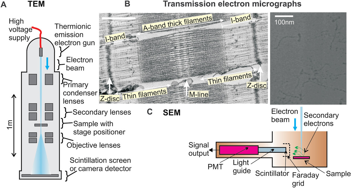
Figure 5.1 Electron microscopy. (a) Schematic of a transmission electron microscope. (b) Typical electron micrograph of a negatively stained section of the muscle tissue (left panel) showing a single myofibril unit in addition to several filamentous structural features of myofibrils and a positively shadowed sample of purified molecules of the molecular motor myosin, also extracted from muscle tissue. (Both from Leake (2001).) (c) Scanning electron microscope (SEM) module schematic.
The relativistic relation between an electron’s rest mass m0, ~9.1 × 10⁻³¹ kg, its momentum p, and its energy given by the energy-momentum equation,
(5.2)But the wavelength of the accelerated electron can be determined from the de Broglie relation that embodies the duality of waves and particles of matter, which on rearranging yields
(5.3)where h is Planck’s constant ~6.62 × 10⁻³⁴ m2 kg s−1. Thus, the usual classical approximation (cited in many textbooks)
(5.4)still holds to within ~10%. Typical accelerated electrons have such matter wave wavelengths of 10−12 to 10−11 m, and waves will exhibit wavelike phenomena such as reflection and diffraction.
The hypothetical spatial resolution Δx of an electron beam probe is diffraction limited in the same sense as discussed previously in Chapter 4 for a visible light photon beam probe, which is determined by the Abbe diffraction limit for circularly symmetrical imaging apertures of ~0.61λ/NA. For a high-resolution (i.e., short wavelength) electron microscope, which might accelerate electrons with ~100 kV, the wavelength λ is ~4 × 10⁻¹² m, whereas the effective numerical aperture, NA, is ~0.01. This would imply an Abbe limit of ~0.2 nm for spatial resolution. However, in practice, the experimental spatial resolution is an order of magnitude worse than would be expected from the Abbe limit at a given wavelength, which is more like 1–2 nm in this instance, mainly due to the limitations of spherical aberration on the electron beam, but also compounded by the finite size of scattering objects used as typical contrast reagents and of spatial distortions to the sample cause by the method of fixation.
5.2.2 Fixing a Sample for Electron Microscopy and Generating Contrast
The ultralow pressures used in standard electron microscopes would result in rapid, uncontrolled vaporization of water from wet biological samples, which would result in sample degradation. The specific methods of sample preparation differ depending on the type of EM imaging employed. For example, cryo-EM (discussed in detail later in this chapter) has distinctly different preparation methods compared to transmission EM and scanning EM techniques. Also, the method of preparation depends of the length scale of the sample—whether one is fixing an entire insect, a cell, a subcellular cell compartment, a macromolecular complex.
Tissue samples prepared for EM are fixed so as to prevent uncontrollable water loss, through either dehydration or freezing, and are often fixed to lock the movement of the biological components in the sample. Chemical fixation is a gradual multistage process of sample dehydration with organic solvents such as ethanol and acetone; incubation with a bivalent aldehyde chemical, typically glutaraldehyde or a modified variant, generates chemical cross-links that are relatively indiscriminate between different biomolecular structures in the sample. The dehydrated, cross-linked sample is then embedded in paraffin wax, which is sliced with a microtome to generate sections of a just a few tens of nanometers of thickness.
The most significant disadvantage with this multistage stage chemical preparation is that it often generates considerable, and sometimes inconsistent, experimental artifacts. Not least of which are volume changes in the sample during dehydration, which potentially affect different parts of a tissue to different extents and therefore lead to sample distortion. Cryofixation (also referred to as “snap freezing”) rapidly cools the sample using a cryogen such as liquid nitrogen or liquid propane instead of chemical fixation, which eliminates some of these problems. Common methods to achieve this include slam freezing, in which the sample is mechanically positioned rapidly against a cold, flat metallic surface, and high-pressure freezing, which is normally achieved at a pressure of ~2000 atm.
A general method to minimize experimental artifacts is to at least aim for robustness in the sample preparation conditions. By this, we mean that the various steps of the sample preparation procedure should be optimized so that the appearance of the ultimate EM images becomes relatively insensitive to small changes in sample preparation, for example, to select a choice of dehydrating reagent that does not result in markedly different images to many other reagents. In other words, this is to optimize the chemical and incubation conditions of sample preparation to be relatively insensitive to their being perturbed.
The key aim of all sample freezing techniques is to vitrify the liquid phases of a biological matter, principally water, to solid to minimize motion of the internal components and to ensure that an amorphous, as opposed to a crystalline, vitreous solid results. The biggest problem is the formation of ice crystals, which occurs if the rate of drop in temperature is less than ~104 K s−1, which in practice means that freezing needs to occur within a few milliseconds. Slam freezing can achieve this on samples, provided they are less than ~10 μm in thickness, while high-pressure freezing can achieve this on larger samples for up to ~200 μm thick.
Cryosubstitution can then be performed on the frozen sample, which involves low-temperature dehydration by substitution of the water components with organic chemical solvents. In essence, the sample temperature is raised very slowly (over a period of a few days typically), and as it melts, the liquid phase water becomes substituted with organic solvents; this can facilitate stable cross-links between large biomolecules driven by hydrophobic forces in the absence of covalent bond cross-links, so eliminating the need for a specific chemical fixation step. Cryoembedding is then performed at temperatures less than –10°C, and samples can be sectioned using a cooled microtome.
Take the example of large protein complexes in the cell membrane. These include membrane-based molecular machines such as the flagellar motor in bacteria that rotates to drive the swimming of bacteria and the ATP synthase molecular machine that generates molecules of ATP (see Chapter 2). Cryofixation is an invaluable preparation approach for these, especially when coupled to a method called “freeze-fracture” or “freeze-etch electron microscopy,” which has been used to gain insight into several structural features of cells and subcellular architectures. Here, the surface of the frozen sample is fractured using the tip of a microtome, which can reveal a random fracture picture of the structural makeup immediately beneath the surface, yielding structural details of the cell membrane and the pattern of integrated membrane proteins.
Aficionados of both cryofixation and chemical fixation in EM report a variety of pros and cons for both methods, for example, on the different respective abilities of each to stabilize the motions of certain cellular components during sample fixation. However, one should be mindful of the fact that although EM has excellent spatial resolution and imaging contrast, all sample preparation methods generate distortions when compared against the relatively less invasive biophysical imaging technique of light microscopy.
5.2.3 Generating Contrast in Electron Microscopy
Biological matter is mostly water and carbon, comprising relatively low-atomic-number elements. This results in a far greater mean free collision path for electrons in carbon compared to high-atomic-number metals. For example, at a 100 kV accelerating voltage, an electron in carbon has a mean free collision path of ~150 nm, whereas in gold, it is ~5 nm. To visualize biological material therefore, a high-atomic-number metal contrast reagent is applied.
Negative staining can be applied on both chemically and cryofixed samples, usually by including a heavy metal contrast reagent such as osmium tetroxide or uranyl acetate dissolved in an organic solvent such as acetone. The contrast reagent preferentially fills the most accessible volumes in the sample (those least occupied by the densest biological matter). This therefore results in a negative image of the sample if the electrons are transmitted onto a suitable detector. This technique can generate excellent contrast between heterogeneous biological matter found in vivo (e.g., illustrated in the case of muscle tissue in Figure 5.1b).
Another contrast reagent incorporation method involves positive staining via metallic shadowing, typically of evaporated platinum. This not only can be applied to relatively large length scale samples (e.g., small whole organisms such as insects) to coat the surface for visualization of backscattered electrons reflected from the metallic coat but is also a common approach applied to visualizing single molecules from visualization of transmitted electrons through the sample. Here, a dilute purified solution of the biomolecules is first sprayed onto a thin sheet of evaporated carbon, which is supported from an EM-grid sample holder. The sample aqueous medium is then dried in a vacuum and platinum is evaporated onto the sample from a low angle <10° as the sample is rotated laterally.
This creates a uniform metallic shadow of topographical features of any single molecules stuck to the surface of the carbon, which are electron dense, generating a high scatter signal from an electron beam, whereas the supporting thin carbon sheet is relatively transparent to electrons and thus results in a “positive” image. Single gold or platinum atoms have a diameter of ~0.3–0.4 nm, but typically, a minimum-sized cluster of atoms in a shadowed single region in a sample might consist of 5–10 such atoms, in which case the real spatial resolution may be worse than expected, after the effects of diffraction and spherical aberration, by a factor of ~2–4.
Metallic shadowing is also used for generating contrast in freeze-fracture samples. Here, larger angles of ~45° are applied in order to reach more recessed surface features compared to single-molecule samples. This method can generate excellent images of the phospholipid bilayer architecture of cell membranes, down to a precision sufficient to visualize single polar head groups of a phospholipid molecule.
Both tissue-/cellular-level samples and single-molecule samples can also be visualized using immunostaining techniques. These involve incubating the sample with a specific antibody, which contains a heavy metal tag of just a few gold atoms. The antibodies will then bind with high affinity to specific molecular features of the sample, thus generating high electron beam attenuation contrast for those regions, often used to complement negative staining. However, a single antibody has a Stokes radius of ~10 nm, which reduces the effective spatial resolution of this method. Recent improvements have involved the development of genetically encoded EM labels for use in correlative light and electron microscopy (CLEM) techniques (discussed later in this chapter).
5.2.4 Transmission Electron Microscopy
Biological samples can be imaged by detecting the intensity of transmitted electrons, in transmission electron microscopy (TEM), or by the backscattered secondary electrons, in scanning electron microscopy (SEM). TEM is valuable for probing cellular morphology in tissues, subcellular architectures, and a range of molecular-level samples. In TEM, the accelerating voltage is ~80–200 kV, capable of generating a wide-field electron beam at the sample of up to several tens of microns in diameter. Contrast reagents are normally used in the form of negative staining, metallic shadowing, or immunostaining. Low-voltage electron microscopy (LVEM) in the range ~0.2–10 kV can also be used in transmission mode. The electron wavelength is larger by a factor of 3–4, which therefore reduces the spatial resolution by the same factor. Also, the mean collision path at these lower electron energies in carbon is more like ~15 nm. This means that the biological sample must be of comparable thickness, that is, sectioned very thinly and consistently; otherwise, insufficient electrons will be transmitted. However, a by-product of this is that additional contrast reagents are not required and thus the data are potentially more physiologically relevant.
Some old machines are still in operation in which transmitted electrons are detected via a phosphor screen of typically zinc sulfide, which can then be imaged onto a CCD camera (in fact some machines in operation still use photographic emulsion film). As time advances, many of these older machines will inevitably become obsolete, though a significant minority are still being used in research laboratories. Most modern machines detect the transmitted electrons directly using optimized CCD pixel arrays, which offer some improvement in avoiding secondary scatter effects of emitted light from a phosphor.
A useful variant of TEM is electron tomography (ET). This involves tilting the biological sample stage over a range of ±60° from the horizontal around the x and y axes of the xy sample plane. This generates different projections of the same sample, which can be reconstructed to generate 3D information. The reconstruction is usually performed in reciprocal space; though there are missing angles due to the finite range of stage tilt permitted, there is a missing wedge of data in the Fourier plane corresponding to these unsampled orientations. There is a reduction in spatial resolution by factor of ~10 compared to conventional TEM at comparable electron energies, but the insight into molecular structures, especially when combined with cryogenic sample conditions (often referred to as cryo-ET, discussed later in this chapter), can be significant.
In principle, 3D information can also be generated through electron holography. Some working designs that utilize adaptations to transmission mode LVEM using electron energies can generate an electron holograph (also known as a Gabor hologram, a Ronchigram) or a nonbiological sample, using, in essence, the same physical principles as those for digital holography in light microscopy discussed previously (Chapter 3). These techniques have yet to find important applications in biophysics, which is ironic since the original concept of holography developed by Dennis Gabor was to improve the spatial resolution achievable in EM by dispensing with the need for electron lenses to focus the beam, which result in the resolution-limiting spherical aberration (Gabor, 1948). The conceived instrument was to be called the “electron interference microscope,” though the practical implementation at the time was not possible since it required a point source of electrons that was technically not achievable with existing technologies. However, a variation of this technique is ptychography, which has made promising progress discussed later in this section.
5.2.5 Scanning Electron Microscopy
SEM is a lower magnification technique compared to TEM and can generate important structural details on the surface of tissues and small organisms at a length scale of more like several tens to hundreds of microns (Figure 5.1c). It uses a lower range of accelerating voltage of ~10–40 kV compared to TEM. The beam is focused onto the sample to generate a confocal volume, similar in egg shape to that of light microscopy but with a lateral diameter of typically only a few nanometers. The beam passes through pairs of scanning electromagnetic coils or paired electrostatic deflector plates, which displace it laterally to scan the confocal electron volume over the sample surface in a raster fashion.
Electrons from this confocal volume lose energy due to scattering and absorption, which extends to a larger interaction volume whose length scale is greater than that of the confocal volume by at least an order of magnitude. Detected electrons from the sample are either those due backscattered/reflected electrons via elastic scattering, or more likely due to secondary electrons due to inelastic scattering. These have relatively low energies <50 eV and result from the absorption and then ejection from a K-shell electron in a scattering atom from the sample. This low energy manifests as a small mean collision path in the sample of only a few nanometers, and so any secondary electrons that are detected ultimately originate very close from the sample surface. Thus, SEM using secondary electron detection generates just a topographical detail of the sample.
Such surface secondary electrons are first accelerated toward an electrically biased grid at ~90° to the electron beam by a few hundred volts and then further toward a phosphor scintillator inside a Faraday cage (also known as a Everhart–Thornley detector), coupled to a photomultiplier tube (PMT) with a higher E-field of ~2 kV potential difference to energize the electrons sufficiently to allow scintillation in the phosphor. The resulting PMT electric current is then used as a metric for the secondary electron intensity. Although SEM in itself is not a 3D technique, the same stage tilting and image reconstruction technology as for transmission ET can be applied to generate 3D information on topographical features.
Rarer elastically backscattered electrons are higher in energy and so can scatter at relatively high angles. The electrons can emerge from anywhere in the sample, and thus, backscattered electron detection is not a topographic determination technique. To detect backscattered electrons and not secondary electrons, similar scintillation PMT detectors can be placed in a ring around the main electron beam (i.e., at relatively high scatter angles), allowing electron backscatter diffraction images to be generated.
The extent of backscatter is dependent on the atomic number of the metal element in the contrast reagent. In principle, this offers the potential to apply differential imaging on the basis of different atomic number components used to stain the sample. This has been applied to a few exceptional multiple length scale investigations, for example, to probe the optic nerve tract by using a nonspecific lead metal stain, which reveals topographic information of the tract from the detected secondary electrons, while using a specific silver metal stain, which targets just the nerve fibers themselves inside the tract. Silver has a higher atomic number than lead and thus backscatter electron detection can be used to image just the localization of the nerve fibers in the same optic nerve tract.
An SEM can, in principle, be modified to operate simultaneously in the transmission mode. This involves implementing detectors below the sample to capture transmitted electrons, as for conventional TEM. Most mainstream EM machines do not operate in this hybrid manner; however, there is a benefit in using transmission scanning electron microscopy since, if used in conjunction with LVEM on unstained samples, it improves the image contrast. Thus, this may serve as a useful control at least against the presence of experimental artifacts caused through chemical staining procedures.
Some SEM machines are also equipped with an x-ray spectrometer. X-ray spectroscopy is discussed in more detail later in this chapter, but in essence, K-shell electron ejection also generates x-rays and their wavelength is dependent on the specific electronic energy levels of the atom involved. It can therefore be used to investigate the elemental makeup of the sample (elemental analysis).
Conventional SEM uses the same high vacuum as TEM. The requirement for dehydrated or frozen samples means that imaging cannot be done under normal “environmental” conditions. However, the environmental scanning electron microscope (ESEM) overcomes this limitation to a large extent. ESEM utilizes the same generic SEM design but implements a modified sample chamber, which allows a higher pressure to be maintained in a humidified environment. The electron beam attenuation in air increases exponentially with the distance as the electron beam must penetrate into the sample; therefore, the key developments in ESEM have been in miniaturization of the sample chamber. Modern ESEM devices often have variable pressure options with Peltier temperature control for the sample chamber, allowing a range of EM modes to be used, with pressures of a few kilopascals being sufficient to prevent water vaporization from wet samples.
5.2.6 Cryo-EM and CryoET
The term cryo-EM is often misused in any EM performed on samples, which have been prepared using cryofixation. However, a better use is for describing EM on a native sample involving no dehydration step at which the sample temperature throughout, not just the fixation step but the entirety of the investigation from sample preparation through to the final imaging acquisition, has been kept below 140 K, which is the vitrification temperature of water, or in other words biological samples with very minimal sample preparation artifacts. These investigations require a specialized cold stage, typically using liquid nitrogen (boiling point 77 K, which allows a stable cold stage of 110 K to be maintained) or, in some advanced machines, liquid helium (boiling point 4 K).
Cryo-EM is particularly useful as a structural biology tool, both using metallic shadowing and negative staining techniques, and can be applied in transmission and scanning modes. For molecular-level structural investigations, cryo-EM is used for superior spatial resolution compared to SEM. However, the absolute level of spatial resolution in raw cryo-TEM molecular reconstructions is still an order of magnitude worse than the definitive atomic-level resolution achievable by the techniques of nuclear magnetic resonance (NMR) and x-ray crystallography. However, improvements in the methods of image analysis in particular mean that cryo-EM in many cases rivals the traditional atomic-level structural biology methods.
For example, the inferior raw spatial resolution of EM compared to the atomistic-level structural biology techniques can be improved by subclass averaging. This operates by categorizing each raw image of a molecular complex into a distinct class of image type, aligning each image within that class and then generating a single average image for each subclass. In the early days of this technique, in fact, close to the turn of the twentieth century, such averaging was performed manually, in a highly precarious and potentially subjective way. However, improvements in modern subclass categorization methods involve principal component analysis of eigenimages (originally described as eigenfaces from its implementation in face recognition software), although there are still potential issues with user-defined thresholds for determining and recognizing subclass features (discussed in Chapter 8).
However, cryo-EM also has some important advantages over x-ray crystallography and NMR, in that it can be applied to molecular complexes that are >250 kDa in summed molecular weight, which is far greater than NMR (~90 kDa maximum) and can be applied to intact large molecular complexes unlike x-ray crystallography, which requires the formation of highly pure crystals, which are too difficult to generate either because they require the presence of a phospholipid bilayer to form stably or because they consist of multiple molecular components. These include not only the large membrane complexes of the flagellar motor and ATP synthase mentioned earlier but also certain essential macromolecular complexes in the cytoplasm such as the intact ribosome and large intact viruses. The ribosome is a particularly good example since the separate components of a ribosome can be purified and structures are determined by x-ray crystallography, whereas to visualize the entirety intact ribosome requires a technique such as cryo-EM.
Electron cryotomography (CryoET) is a specific application of cryo-EM for which 3D images can be reconstructed from multiple 2D images of a sample obtained by tilting over a range of orientations up to a limit of around 70˚. Since the electron propagation distance though the sample increases during tilting, this imposes a practical sample thickness upper limit to avoid significant electron beam attenuation, typically around 0.5 µm. Many CryoET studies to date have thus focused on unicellular microbes and viruses, and macromolecular complexes, though thinning of larger samples can be performed using focused ion beam (FIB) milling, in addition to normal cryo-sectioning. CryoET may also be combined with fluorescence microscopy methods to generate more specificity for identifying cellular structures, using similar correlative approaches to those described in Section 5.2.7.
5.2.7 Correlative Light and Electron Microscopy
Correlative light and electron microscopy (CLEM) combines the advantages of the time-resolved fluorescence microscopy on live cellular material with the higher spatial resolution achievable with EM. As we discussed in Chapter 4, fluorescence microscopy offers a minimally invasive high-contrast tool, which can be used on live-cell samples to monitor dynamic biological processes to a precision of single molecules. However, the diffraction-limited lateral spatial resolution of conventional far-field fluorescence microscopes is ~200–300 nm. This can be improved by an order of magnitude by superresolution techniques but is still another order of magnitude inferior to TEM. But TEM, in turn, suffers the prime disadvantage of being a dead sample technique. CLEM has made important advances in developing methods to combine some of the advantages of both the approaches.
CLEM can utilize a variety of different stains, which can specifically label a biological structure in the sample but be visible in both fluorescence microscopy and TEM. These stains include novel hybrid probes such as fluorescent derivatives of nanogold particles and also quantum dots, since the cadmium atoms at the QD core are electron dense. FlAsH and ReAsH can also be utilized by using a specific photon-induced oxidation reaction with a chemical called “diaminobenzidine” (DAB), which causes the DAB to polymerize. In its polymeric state, it can react rapidly with osmium used in negative staining. Secondary antibodies used for immunofluorescence can also be labeled with a fluorophore called “eosin,” which is also a substrate that is sensitive to photooxidation of DAB.
The most promising developments involve the use of cryo-EM and genetically encoded fluorescent protein labels. The use of chemical fixation affects the ability of fluorescent proteins to fluoresce; although some fixative recipes exist, which affect fluorescent proteins less, there is still a drop in fluorescence efficiency. However, the rapid freezing methods of cryofixation methods have shown promise in preserving the photophysics of fluorescent proteins. Although fluorescent proteins show no clear direct sensitivity to DAB, there have been some positive results using secondary immunolabeling of green fluorescent protein (GFP) itself. The state of the art is the mini-singlet oxygen generator (miniSOG), which is a fluorescent flavoprotein engineered from a phototropin protein from the plant of genus Arabidopsis (used as a common model organism, see Chapter 7). MiniSOG contains only 106 amino acids, roughly half as many as GFP, and illumination generates enough singlet oxygen to locally catalyze the polymerization of DAB, which is then resolvable by EM.
The ability to image the same region of a sample is facilitated by gridded or patterned coverslips, which aid in pattern recognition between light and electron microscopes. But a key development for CLEM has been the reduction in the time taken to transfer a sample between the two modes of microscopy. Automated fast-freezing systems can now allow samples to be imaged by fluorescence microscopy, cryofixed within ~4 s, and then imaged immediately afterward using TEM.
5.2.8 Electron Diffraction Techniques
Electron diffraction works on the same scattering principles as for light diffraction discussed previously in Chapters 3 and 4; however, the incident beam of accelerated electrons interacts far more strongly with matter. This means that 3D crystals are largely opaque to electron beams. However, 2D spatially periodic cellular structures can generate a strong emergent scatter pattern, which can be used to determine structural details. Since electron beams can be focused using electromagnetic lenses, the diffraction pattern retains phase information from the sample in much the same way as focused rays of light in optical microscopy. This offers an advantage over x-ray diffraction for which phase information has to be inferred indirectly (discussed later in this chapter).
A key biophysical application of electron diffraction is determining structural details of lipid arrays and membrane proteins, for which 3D crystals are difficult to manufacture, which is a requirement for x-ray crystallography. Close-packed 2D lipid–protein arrays are feasible to make, to determine the spacing of periodic biological structures in the sample, using both backscattered electrons in Bragg reflection experiments and transmitted electrons. Electrons incident on a sample having periodic features over a characteristic length scale db can generate backscattered electrons (also known as “Bragg reflection” or “Bragg diffraction”) by an angle θb from the normal. Since the backscattered electrons are coherent, they can interfere, such that the condition for constructive interference generates an nth order intensity maxima, which are given by Bragg’s law, where n is a positive integer:
(5.5)Primary electrons may, of course, also be transmitted through the sample at an angle θt from the normal due to electron diffraction through periodic layer features of length scale dt, with the condition for constructive interference being
(5.6)Selected area diffraction is often used for electron diffraction, in which a metal plate containing different aperture sizes can be moved to illuminate different sizes and regions of the sample. This is important in heterogeneous samples; these are potentially polycrystalline, which can result in difficult interpretations of electron diffraction patterns if more than one equivalent periodic structure is present. If it is possible to spatially delimit the area of illumination to just one diffracting periodic region, this problem can often be eradicated. However, the strong interaction with matter of the electron beam confers a significant danger of radiation damage of the sample, and consequently, samples need to be cooled using liquid nitrogen or sometimes liquid helium.
Electron diffraction can also be used in ptychographic EM (Humphry et al., 2012). The key physical principles of ptychographic diffractive imaging for EM are the same as those discussed previously for light microscopy in Chapter 4. In essence, physical lenses used for imaging can be replaced by an inverse Fourier transform of the diffraction data detected from the sample.
The same method has been applied in a bespoke setup using relatively low-energy 30 kV electrons to form a transmitted electron diffraction image. By modifying an SEM, the primary electron is defocused to generate a broader 20–40 nm illumination patch on the sample. The effects of spherical aberration by the objective electron lens, which normally focuses the beam onto the sample, are largely eradiated since it is used simply to concentrate the electron beam into a delimited region of the sample, as opposed to acting as an imaging component.
A CCD detector is located below the sample to detect the transmitted diffracted electrons (the diffraction pattern formed is a type of a Gabor hologram), which is combined with a much stronger signal from transmitted nonscattered electrons. The phases from a scattering object can be recovered in a similar way using the ptychographic iterative engine (PIE) algorithm as for optical ptychography, since the scanned electron beam moves over the sample to generate overlap.
Measuring the diffraction intensity with the CCD and calculating the respective phases in principle would allow 3D reconstruction of the sample. However, thus far, samples have been limited to being relatively thin. But even so, this method, in eradicating spherical aberration limits, has improved spatial resolution at 30 kV by a factor of ~5 compared to equivalent energies in a conventional TEM.
5.3 X-Ray Tools
X-rays (originally known as “Röntgen rays” in Germany where they were first discovered) are composed of high-energy electromagnetic waves, which have a typical range of wavelength of ~0.02–10 nm. This is very similar to the length scale for the separation of individual atoms in a biological molecule and also for the size of certain larger scale periodic features at the level of molecular complexes and higher length-scale molecular structures, which makes x-rays ideal probes of biomolecular structure. X-ray diffraction, in particular, is an invaluable biophysical tool for determining molecular structures—in excess of 90% of all known molecular structures that have been determined using x-ray diffraction techniques, compared to ~10% by NMR and <1% by EM methods, at the time of writing.
5.3.1 X-Ray Generation
In some research laboratories in the world, x-rays are still generated from a relatively small x-ray tube beam generator, which can fit into a typical small research lab (Figure 5.2a). This device generates electrons from a hot filament (often made from tungsten but also thorium and rhenium compounds) in a similar way to an electron microscope using thermionic emission but accelerates these electrons using high voltages of typically ~20–150 kV to impact onto a metal target plate embedded into a rotating anode. Rotation, at a rate of 100–200 Hz, increases the effective surface area of the metal target to distribute the high heat generated over a greater area. The target is usually composed of either copper or molybdenum, though tungsten, chromium, and iron are also sometimes used. The high energy of the electrons can be sufficient to displace atomic electrons from their atomic orbitals resulting in x-ray emission, either through a Bremsstrahlung mechanism (Figure 5.2b), which results in a continuous x-ray emission spectrum, or x-ray fluorescence, which generates emission peaks at distinct wavelengths.
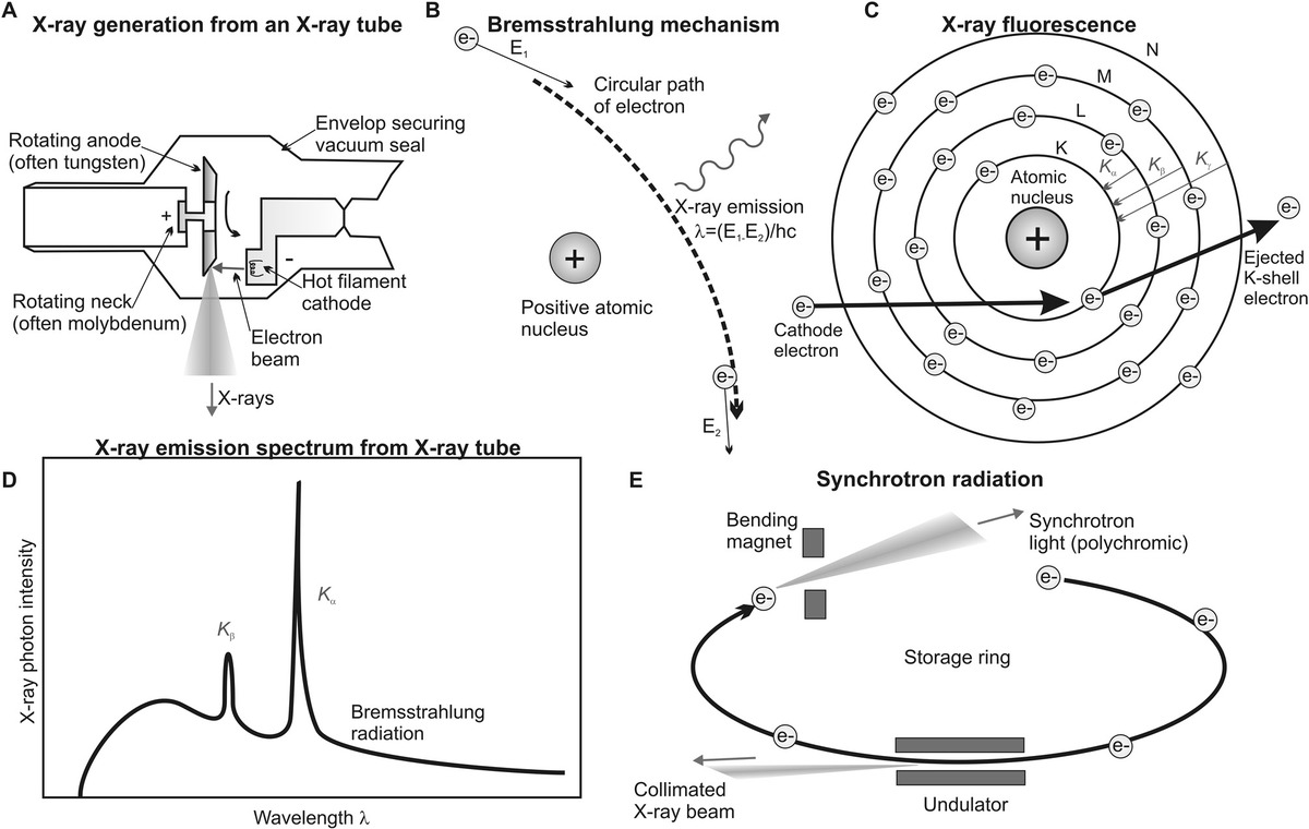
Figure 5.2 X-ray generation. (a) X-ray tube, with rotating anode. (b) Mechanism of x-ray generation from the Bremsstrahlung mechanism in which the energy lost by an electron accelerating round a positively charged high-atomic-number nucleus is emitted as x-rays. (c) Process of x-ray fluorescence following ejection of a core shell electron followed by higher energy shell electrons filling this vacancy, with the energy difference emitted at distinct wavelengths, which can be seen (d) overlaid as peaks on the Bremsstrahlung continuum x-ray spectrum. (e) Intense x-rays may also be generated from a synchrotron facility.
In x-ray fluorescence, incident electrons can have sufficient energy to displace ground-state electrons from the K-shell (i.e., 1s orbital) to generate metal ions (Figure 5.2c). This creates a vacancy in the K-shell, which can be filled by higher-energy electrons from the L (2p orbital) or M (3p orbital) shells, coupled to the fluorescence emission of an x-ray photon of energy equal to the energy difference between these K–L and K–M levels minus any vibrational energy losses of the excited state electron as per the fluorescence mechanism described for optical microscopy (see Chapter 3). This gives rise to Kα (transition from principal quantum number n = 2–1) and less intense Kβ (transition from principal quantum number n = 3–1) x-ray emission lines, respectively, at a wavelength of ~10−10 m (see Table 5.1 for typical wavelengths for Kα). Other shell transitions are possible to the n = 2 level, or L-shells are designated as L x-rays (e.g., n = 3 → 2 is Lα, n = 4 → 2 is Lβ, etc.), but in general, all but the most intense Kα transitions are filtered out from the final emission output from an x-ray tube collected at right angles to the incident electron beam.
| Element | Kαλ (nm) |
|---|---|
| Mo | 0.071 |
| Cu | 0.154 |
| Co | 0.179 |
| Fe | 0.194 |
| Cr | 0.229 |
| Al | 0.834 |
The choice of target in an x-ray tube is a trade-off against the x-ray emission wavelengths desired, the intensity of Kα emission lines, and the target metal having a sufficiently high melting point (since ~99% of the energy from the accelerated electrons is actually converted into heat). Melting point has no clear overall trend across the periodic table, though there is some periodicity to melting point with the atomic number Z and all of the common target metals used are clustered into regions of high melting point on the periodic table. In terms of wavelength of the emission lines, this can be modeled by Moseley’s law, which predicts that the frequency ν of emission scales closely to ~Z2:
(5.7)where k1 and k2 are constants relating to the type of electron shell transition; however, for all Kα transitions k1 = k2 and the equation can be rewritten as
(5.8)The alternative x-ray generation mechanism to x-ray fluorescence is that which produces Bremsstrahlung radiation. Bremsstrahlung radiation is a continuum of electromagnetic wave emission output across a range of wavelengths. When a charged particle is slowed down by the effects of other nearby charged particles, some of the lost kinetic energy can be converted into an emitted photon of Bremsstrahlung radiation. In the raw output from the metal target in an x-ray tube, this emission is present as a background underlying the x-ray fluorescence emission peaks (Figure 5.2d), though in most modern biophysical applications, Bremsstrahlung radiation is filtered out.
Most x-rays generated for use in biophysical research today are generated from a synchrotron. The principle of generating synchrotron radiation is similar to that of a cyclotron; in that, it involves accelerating charged particles using radiofrequency voltages and multiple electromagnet B-field deflectors to generate circular motion, here of an electron (Figure 5.2e). These bending magnet deflectors alter the path of electrons in the storage ring. The theory of synchrotron radiation is nontrivial but is confirmed both in classical physics and at the quantum mechanical levels. In essence, a curved trajectory of a charged particle results in warping of the shape of the electric dipole force field to produce a strongly forward peaked distribution of electromagnetic radiation, which is highly collimated; this is synchrotron radiation.
However, synchrotrons use radiofrequency (f) values that, unlike cyclotrons, are not fixed and also operate over much larger diameters than the few tens of meters of a cyclotron, more typically a few hundred meters. The United States has several large synchrotron facilities including the National Synchrotron Light Source at Brookhaven, with the United Kingdom also investing substantial funds in the DIAMOND synchrotron national facility, with 100 other synchrotron facilities around the world, at the time of writing. Note the largest particle accelerator as such, though not explicitly designed as a synchrotron source of x-rays, is 27 km in diameter, which is the Large Hadron Collider near Geneva, Switzerland.
Equating magnetic and centripetal forces on an electron of mass m and charge q, traveling at speed v with kinetic energy E in a circular orbit of radius r implies simply
(5.9)Thus, f is independent of v, assuming nonrelativistic effects, which is the case for cyclotrons. Synchrotrons have larger values of r than cyclotrons and therefore greater values of E, which can exceed 20 MeV after which noticeable relativistic effects occur; thus, f must be varied with v to produce a stable circular beam.
A synchrotron is a large-scale infrastructure facility but produces brighter beams than x-ray tubes, with a greater potential range of wavelength ultimately permitting greater spatial resolution. The use of major synchrotron facilities for providing dedicated x-ray beamlines for crystallography has increased enormously in recent years. In the two decades, since 1995, the number of molecular structures solved using x-ray crystallography, which were deposited each year in the Protein Data Bank archive (see Chapter 7) from nonsynchrotron x-ray crystallography has remained roughly constant at ~1000 structures every year, whereas those solved using synchrotron x-ray sources has increased by a factor of ~20 over the same period.
Synchrotrons can generate a continuum of highly collimated, intense radiation from lower energy infrared (~10−6 m wavelength) up to a much higher energy hard x-rays (10−12 m wavelength). Their output is thus described as polychromatic. The spectral output from a typical x-ray tube is narrower at a wavelength of ~10−11 m, but both synchrotron x-ray and x-ray tube will often propagate through a monochromator to select a much narrower range of wavelength from the continuum.
Monochromatic x-rays simplify data processing significance and improve the effective resolution and signal-to-noise ratio of the probe beam, as well as minimize damage to the sample from extraneous satellite lines. An x-ray monochromator typically consists of a quartz (SiO2) crystal, often fashioned into a cylindrical geometry, which results in constructive interference at specific angles on for a very narrow range of wavelength due to Bragg reflection at adjacent crystal planes. For a small region of the crystal, the difference in optical path length between the backscattered rays emerging at an angle θ from two adjacent layers, which are separated by a spacing d of an x-ray scattering sample is 2d sin θ, and so the condition for constructive interference is that this difference is equal to a whole integer number n of wavelengths λ, hence 2d sin θ = nλ. Quartz has a rhombohedral lattice with an interlayer spacing of d = 0.425 nm; the Ka line of aluminum has a wavelength of λ = 0.834 nm; therefore, this specific beam can be generated at an angle of θ = 78.5°. The typical bandwidth of a monochromatic beam is ~10−12 m.
A recent source of x-rays for biophysics research has been from the x-ray free-electron laser (XFEL). Although currently not being in sufficient mainstream use to act as a direct alternative to synchrotron-derived x-rays, the XFEL may enable a new range of experiments not possible with synchrotron beams. With x-ray tubes and conventional synchrotron radiation, the x-ray source is largely incoherent, that is, a random distribution of phases of the output photons. However, high-energy synchrotron electrons can be made to emit coherently either if electrons bunch together over a length scale, which is significantly shorter than the wavelength of their emitted radiation bunch that is short with respect to the radiation wavelength, or if the electron density in a given bunch of electrons is modulated with the same frequency as the emitted synchrotron radiation wavelength. For x-rays, it is too challenging currently to directly produce sufficiently small electron bunches; however, electron bunch modulation is now technically feasible and is the basis of the XFEL.
In essence, a linear electron beam is generated using high voltage to give relativistic speeds, either from an output port of a conventional synchrotron or from using a linear accelerator (LINAC) design. LINACs have a disadvantage over synchrotrons in requiring greater straight-line distances over which to operate (e.g., the Stanford LINAC, which currently operates as the world’s only superconducting LINAC, is ~3 km in length), but have an advantage in that less energy from accelerated particles is unavoidably lost as synchrotron radiation. The accelerated electron beam is propagated through an undulator consisting of a periodic arrangement of magnets transverse to the beam, with adjacent magnets on each side of the beam arranged with alternating pole geometries (Figure 5.3a) and having a period length parallel to the beam axis of usually a few tens of millimeters, which generate a B-field amplitude of ~1 T. This causes a wiggle on the electron beam to generate a sinusoidal electron path around the main beam axis such that the high curvature at the peak sinusoidal amplitudes results in the release of synchrotron radiation generated toward the forward beam axis direction, which is highly coherent. However, unlike a visible light laser, there are no equivalent mirror for x-rays, which could be used to generate a resonant cavity (i.e., to reflect the synchrotron radiation back along the undulator thereby amplifying the x-ray laser output) so instead an extended undulator length is used up to a few meters.
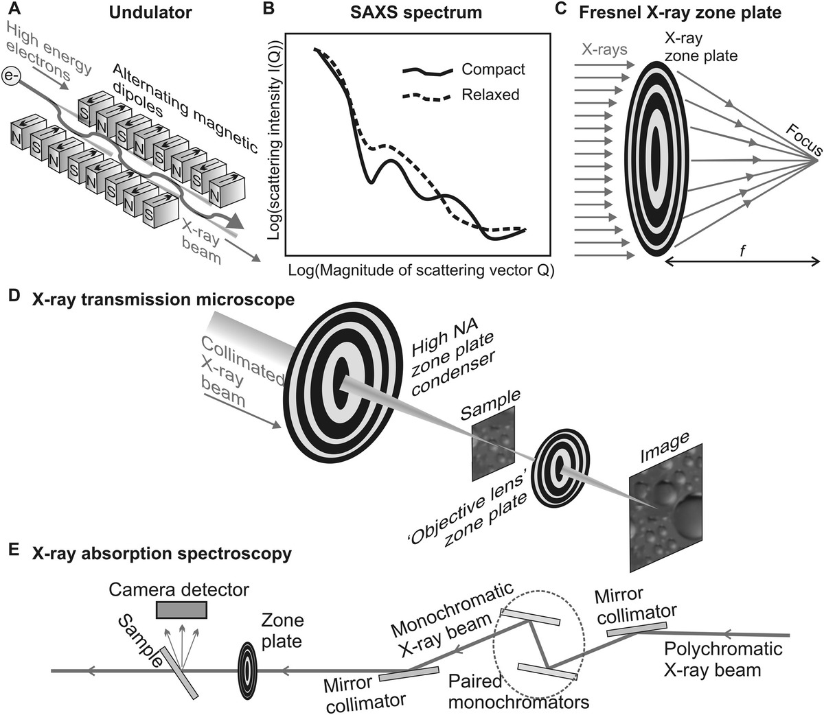
Figure 5.3 X-ray applications. (a) Undulator, used in a LINAC, x-ray free-electron laser, or as a module in a synchrotron, which generates a periodic wiggle in the electron beam resulting in an amplified x-ray emission. (b) Schematic of a typical SAXS spectrum of a protein complex in a solution, which allows quantitative discrimination between, for example, two different molecular conformational states. (c) Fresnel zone plate that acts as a “lens” for x-rays and can be used in (d) and x-ray transmission microscope, as well as (e) and x-ray absorption spectrometer.
The wavelength range of an XFEL currently is ~10−10 to 10−9 m, with an average brightness ~100 times greater than the most advanced synchrotron sources. However, since the magnets in the undulator have a well-defined periodicity, the laser output is pulsed, with a pulse duration of ~10−13 s, compared to an equivalent pulse duration of ~10−11 s for a synchrotron source, and so the peak brightness of the XFEL can be several orders of magnitude greater. This ultrashort pulse duration is having a significant impact into conventional x-ray crystallography for determining the structure of biomolecules in reducing the sample radiation damage dramatically—the rapid pulse x-ray beam results in diffraction before destruction.
One such application is in X-ray pump–probe experiments. Here, ultrashort optical laser pulses are directed onto crystal to generate transient states of matter, which can subsequently be probed by hard x-rays. The fast pump rate of the XFEL (pulse duration of a few tens of femtoseconds) enables time-resolved investigation, that is, more than one shot to be made on the same crystal to monitor rapid structural dynamics. Also, as discussed in the following, there is significant benefit from having a coherent x-ray source in obtaining direct phase information from x-ray scattering atoms in a biomolecule sample.
5.3.2 X-Ray Diffraction by Crystals
A 3D crystal is composed of a regular, periodic arrangement of several thousand individual molecules. When a beam of x-ray photons propagates through such a crystal, the beam is diffracted due to interference between backscattered x-rays from the different crystal layers. The scattering effect is due primarily to Thompson elastic scattering, which results from the interaction of an x-ray photon with a free outer shell valence electron, unlike electron scattering, which is from atomic nuclei, and is also influenced mainly by the electron orbital density. The angle of an emergent diffracted x-ray beam is inversely related to the length of separation within the periodic structures involved in the scattering, in exactly the same way that was discussed for electron diffraction, modeled by Bragg’s law discussed previously for electron diffraction.
The smallest repeating structure in a crystal is called the “unit cell,” and for the simplest crystal shape, which is that of an ideal cubic crystal, the unit cell can be characterized by a crystal lattice parameter a0 and the interplanar spacings, dhkl of planes, which are labeled by Miller indices (h, k, l):
(5.10)Similar relations for dhkl exist for each different-shaped unit cells in a crystal (e.g., orthorhombic, tetragonal, hexagonal). As an example, for the cubic unit cell, the diffractive intensity maxima generated at angle θhkl satisfies
(5.11)Broadly, there are three practical methods for observing clear diffraction peaks from crystalline samples. Some samples may consist of heterogeneous crystals, that is, are polycrystalline, and the Debye–Scherrer method uses a monochromatic source of x-rays, which can determine the distribution of interlayer spacing. The Laue method uses instead a polychromatic x-ray source, which produces a range of different diffraction peaks as a function of wavelength that can be used to determine the interlay spacing distribution provided the sample consists of just a single crystal (the combination of a polycrystalline sample with a polychromatic x-ray source generates a diffraction pattern, which is difficult to interpret in terms of the underlying distribution of interlayer spacings). The most useful approach is the single-crystal monochromatic radiation method, which generates the most easily interpreted diffraction pattern concerning interlayer spacings.
The intensity of the diffraction pattern can be modeled as the Fourier transform of a function called the “Patterson function,” which characterizes the spatial distribution of electron density in the crystal. The pattern of all the scattered rays appears as periodic spots of varying intensity and may be recorded behind the crystal using a CCD. Typically, the crystal will be rotated on a stable mount so that diffraction patterns can be collated from all possible orientations. However, growing a crystal from a given type of biomolecule with minimal imperfections can be technically nontrivial (see Chapter 7). To maximize the effective signal-to-noise ratio of the scattered intensity from a crystal, there is a benefit of growing one large crystal as opposed to multiple smaller ones, and this larger scale is also a benefit due to radiation damage destroying many smaller crystals. In many examples of biomolecules, it is simply not possible to grow stable crystals.
The intensity and spacing of the spots in the diffraction patterns is the 2D projection of the Fourier transform of spatial coordinates of the scattering atoms. The coordinates can be reconstructed using intensive computational analysis, hence, to solve the molecular structure, with a typical resolution being quoted as a few angstroms (which equals 10−10 m, useful since it is of a comparable length scale to covalent bonds). However, an essential additional requirement in this analysis is information concerning the phase of scattered rays. For conventional x-ray crystallography, which uses either incoherent x-ray tube or synchrotron radiation, the intensity and position of the maxima in the diffraction pattern alone do not provide this, since there is no x-ray “lens” as such to form a direct image that can be done using visible light wavelengths, for example.
Crystallographers refer to this as the phase problem, and this phase information is often then obtained indirectly using a variety of additional methods such as doping the crystals with heavy metals at specific sites, which have known phase relationships. Phase information is normally generated by using iterative computational methods, the most common being the hybrid input–output algorithm (HIO algorithm). Here, a Fourier transformation and an inverse Fourier transformation are iteratively applied to shift between real space and reciprocal space under specific boundary conditions in each. This approach is also coupled to oversampling by sampling the diffraction intensities in each dimension of reciprocal space at an interval of at least twice as fine as the Bragg peak frequency (the highest spatial frequency detected for a diffraction peak in reciprocal space). For the real space part of structural refinement, molecular dynamics and structural modeling/validation are also widely used (see Chapter 8).
X-ray crystallography has been at the heart of the development of modern biophysics. For example, the first biomolecule structure solved was that of cholesterol as early as 1937 by Dorothy Hodgkin, and the first protein structures solved were myoglobin in 1958 (John Kendrew and others) followed soon after by hemoglobin in 1959 (Max Perutz and others). There are important weaknesses to the method, which should be noted, however. A key disadvantage of the technique, as with all techniques of diffraction, is that it requires an often artificially tightly packed spatial ordering of molecules, which is intrinsically nonphysiological. In addition, the approach is reliant upon being able to manufacture highly pure crystals, which are often relatively large (typically a few tenths of a millimeters long, containing ~1015 molecules), which thus limits the real molecular heterogeneity that can be examined since the diffraction information obtained relates to mean ensemble interference properties from a given single crystal. In some cases, smaller crystals approaching a few microns of length scale can be generated.
Also, the crystal-manufacturing process is technically nontrivial, and many important biomolecules, which are integrated into cell membranes, are difficult, if not impossible, to crystallize due to the requirements of added solvating detergents affecting the process. In addition, since the scattering is due to interaction with regions of high electron density, the positions of hydrogen atoms in a structure cannot be observed by this method directly since the electron density is too low, but rather, need to be inferred from knowledge of typical bond lengths. Just as important, however, is the lack of real time-resolved information of a biological structure—a crystal is very much a locked state. Since dynamics are essential to biological processes, this is a significant disadvantage, although efforts can be made to infer dynamics by investigating a variety of different locked intermediate states using crystallographic methods. Diffusing x-ray scattering from amorphous samples (see in the following text) can circumvent some of the issues encountered earlier regarding the use of crystals, since they can reveal some information about protein dynamics, albeit under nonphysiological conditions.
5.3.3 X-Ray Diffraction by Noncrystalline Samples
X-ray diffraction can also be performed on a powder if it is not possible to grow sufficiently large 3D crystals. A suitable powder is not entirely amorphous but is composed of multiple small individual crystals with a random orientation. Therefore, all possible Bragg diffractions can be exhibited in the powder pattern. However, the relative positions and intensities of peaks in the observed diffraction pattern can be used to estimate the interplanar spacings. Similarly, biological fibers can be subjected to x-ray diffraction measurements if there is sufficient spatial periodicity. For example, muscle fibers have repeating subunits arranged periodically in one dimension parallel to the long axis of the fiber. This approach was also used to great effect in solving the double-helical structure of DNA from the work of Crick, Franklin, Wilkins, and Watson in 1953.
In small-angle x-ray scattering (SAXS), a 3D crystalline sample is not needed, and the technique is particularly useful for exploring the longer scale periodic features encountered in many biological fibers. The range of scattered angles explored is small (typically <10°) with a typical spatial resolution of ~1–25 nm. It is used to infer the spacing of relatively large-scale structures up to ~150 nm (e.g., to study periodic features in muscle fibers). The scatter signal is relatively weak compared to higher angle scattering methods of x-ray crystallography and so a strong synchrotron beamline is generally used. SAXS does not generate atomistic-level structural information like x-ray crystallography or NMR, but it can determine structures, which are coarser grained by an order of magnitude in a matter of days for biological structures, which span a much wider range of size and mass.
SAXS is performed using an x-ray wavelength of ~0.15 nm, directing the beam to a solution of the biomolecular structure, and the emergent scatter angle θ and beam intensity I are recorded. The magnitude of the scattering vector Q = (4π/k)sin(θ/2), the formulation identical to that discussed for static light scattering previously (see Chapter 4), is normally plotted as a function of I (Figure 5.3b) and the position and sizes and the typically broad peaks in this curve are used to infer the size and extent of spatial periodicity values from the sample. The same level of analysis for determining radius of gyration can also be performed for static light scattering, also including information about the coarse shape of periodic scattering objects in the sample, but SAXS also has sufficiently high spatial resolution to investigate different molecular states of the same complexes, for example, to be able to discriminate between different conformational states of the same enzyme provided the whole sample solution is sufficiently synchronized. And, being in solution, it also offers significant potential for monitoring time-resolved changes to molecular structure, which 3D x-ray crystallography cannot. The use of coherent x-rays as available from XFEL can generate the speckled interference patterns from SAXS investigations, which can be used to generate phase information directly from the sample in much the same way as for XFEL on 2D crystal arrays.
SAXS, like 3D x-ray crystallography, utilizes elastic x-ray photon scattering. Inelastic scattering is also possible, for which the wavelength of the emergent x-rays is greater than the incident beam (i.e., the scattered beam has a lower energy). Here, some portion of the incident photon energy is transferred from the beam to energize a process in the sample, for example, to excite an inner shell electron to a higher energy level. This is not directly useful in determining atomic-level structures but has been utilized in the form of resonant inelastic soft x-ray scattering (RIXS), which can be applied to a solution of biomolecules in the same way as SAXS.
However, since RIXS is often associated with changes to the energy state of atomic electrons, it is often used in biophysical investigations that involve changes to the oxidation state of transition metal atoms in electron-carrier enzymes, for example, those used in oxidative phosphorylation and photosynthesis (see Chapter 2) but has also been applied to biological questions including solvation effects in chemoreceptors and studying the dynamics of phospholipid bilayers.
5.3.4 X-Ray Microscopy Methods
X-ray microscopy methods have been developed both for transmission and scanning modes similar to the principles of EM and optical microscopy. However, the principal challenge is how to focus x-rays, since no equivalent lens as such exists as for the transparent glass lenses of optical microscopy or the electromagnetic/electrostatic lenses of EM. The solution is to use zone plates (Figure 5.3c), also known as Fresnel zone plates, which utilize diffraction for focusing instead of reflection or refraction.
Zone plates are micro- or nanofabricated concentric ring structures known as Fresnel zones, which alternate between being opaque and transparent. They can be used for focusing across the electromagnetic spectrum, and in fact for any general waveform such as sounds waves but are particularly valuable for x-ray focusing. X-rays hitting the zone plate will diffract around the opaque zones. The zone spacing between the rings is configured to allow diffracted light to constructively interfere only at a desired focus. The condition for this is
(5.12)where
- rn is the radius of the switch position between the nth opaque and transparent zones from the center of the zone plate, such that n is a positive integer
- f is the effective focal length of the zone plate
Analogous to the diffraction resolution limit in optical microscopy (Chapter 4), the smallest resolvable object feature length Δx when using a zone plate limit is given by
(5.13)Therefore, the resolution limit is really determined by the precision of the micro-/nanofabrication. At the time of writing, the current reliable limit is ~12 nm.
Typical designs for a transmission x-ray microscope (TXM) and a scanning transmission x-ray microscope (STXM) are shown in Figure 5.3d. “Soft” x-rays are used typically from a collimated synchrotron source, of wavelength ~10–20 nm. The TXM uses two zone plates as equivalent condenser and objective “lenses” to form a 2D image on a camera detector, whereas the STXM typically utilizes just a single zone plate to focus the x-ray beam onto a sample. As a robust biophysical technique, x-ray microscopy is still in its infancy, but it has been tested on single-cell samples.
An alternative to using physical focusing methods of x-rays with zone plates is to perform numerical focusing through similar techniques of coherent x-ray diffraction imaging (CXDI or CDI) and ptychography (which was discussed previously as part of optical microscopy techniques in Chapter 4). CXDI involves a highly coherent incident beam of synchrotron x-rays, which scatter from the sample and generate a diffraction pattern, which is recorded by a camera. This raw diffraction pattern is used to reconstruct the image of the sample through a Fourier transform on the intensity data combined with computational iterative phase recovery algorithms to recover the phase information due to the lack of sufficient coherence used in synchrotron radiation. In effect, a computer performs the job of an equivalent objective lens to convert reciprocal space data into a real space image. The main advantage of CXDI is that it does not require lenses to focus the beam so that the measurements are not affected by aberrations in the zone plates but rather is only limited by diffraction and the x-ray intensity. Although not yet a mainstream biophysical technique, the superior penetration power of x-rays combined with their small wavelength and thus high spatial resolution has realistic potential for future studies of complex biological samples (see Thibault et al., 2008). A future potential for these techniques lies in time-resolved x-ray imaging.
5.3.5 X-Ray Spectroscopy
An incident x-ray photon can have sufficient energy to eject a core electron through the photoelectric effect, resulting in the appearance of significant absorption edges in the spectra of transmitted photons through the sample, which correspond to the binding energies for an electron in different respective shells (K, L, M, etc.). This subatomic process can involve subsequent fluorescence emission analogous to that exhibited in light microscopy (Chapter 3); if an excited electron undergoes vibrational losses prior to returning to its ground state, it results in radiative x-ray fluorescence emission of a photon of slightly longer wavelength than the incident photon. Also, when the ejection of the core inner shell electrons occurs, it results in higher energy outer shell electrons dropping to these lower energy vacant states with a resultant radiative emission of a secondary x-ray photon whose energy is the difference between the binding energies of the two electronic levels. The position and intensity of these absorption and emission peak as a function of photon wavelength, constituting a unique fingerprint for the host atom in question, and thus, x-ray absorption spectroscopy (XAS) (also known variously as very similar/identical techniques of energy-dispersive x-ray spectroscopy, energy-dispersive x-ray analysis, and simply x-ray spectroscopy) is a useful biophysical tool for determining the makeup of individual elements in a sample, that is, performing elemental analysis.
X-ray absorption spectra of relevance to biological questions can be categorized into x-ray absorption near edge structure, which generates data concerning the electronic “oxidation state” of an atom and the spatial geometry of its molecular orbitals, and extended x-ray absorption fine structure, which generates information about the local environment of a metal atom’s binding sites (for an accessible review, see Ortega et al., 2012). The penetration of lower energy secondary x-rays (wavelengths >1 nm) through air is significantly worse than those of higher energy secondary x-rays (wavelength <1 nm). This characteristic wavelength for K-line transitions varies as ~(Z − 1)2 as predicated by Moseley’s law, and the ~1 nm cutoff occurs at around Z = 12 for magnesium. Thus, most metals generate detectable secondary x-rays, which facilitate metal elemental analysis. Of special relevance are metal-binding proteins, or metalloproteins, and XAS can probe details such as the type of neighboring atoms, how many bonds are formed between them, over what distances, and others. This is a particularly attractive feature of the technique, since proteins containing metal ions actually constitute more than one-third of all known proteins.
A schematic of a typical setup is shown in Figure 5.3e, utilizing a polychromatic synchrotron x-ray source, which generates a suitably intense and collimated beam required for XAS. Normally, hard x-rays are used, with a monochromator then utilized to scan through a typical wavelength range of ~0.6–6 nm. Samples, which can include cultures of cells but more typically consist of high concentrations (~0.5 mM) of protein, need to be cryofixed to a glassy frozen state to stabilize thermal disorder and minimize sample radiation damage. But measurements can at least be performed in a hydrated environment, which increases its physiological relevance.
A standard XAS investigation measures the absorption coefficient as a function of incident wavelength, characterized by the simple Beer–Lambert law (see Chapter 3) from measuring the transmission of x-rays through the sample. However, this transmission mode has too low a sensitivity for the often meager concentration of metals found in many biological materials, and in this instance, x-ray fluorescence emission is a better metric, with the detector position at 90° from the incident beam. Detectors are typically based on doped semiconductor designs such that the absorption of an x-ray photon at a p–i–n junction of PIN diodes (where i is an insulating layer between positive p and negative n doped regions) creates a hotspot of electron–hole pairs, which can be detected as a voltage pulse.
X-ray photoelectron spectroscopy (XPS) is an alternative technique to XAS. A competing mechanism to X-fluorescence following absorption of an x-ray photon by an atom is the emission of a so-called Auger electron—the term Auger electron spectroscopy is synonymous with XPS, and often the technique is abbreviated simply to electron spectroscopy. Here, low-energy x-rays, either from an x-ray tube or synchrotron source, are used to stimulate the photoelectric effect in sample atoms, and these photoelectrons are detected directly by a high-resolution electron spectrometer, and electron intensity is determined as a function of energy. The penetration distance of photoelectrons is ~10 nm in a sample, and so XPS renders surface information from a sample, in addition to requiring high-vacuum conditions between the sample and detector. XPS is less sensitive than XAS with therefore more limited application, but as a tool potentially offers advantages over XAS in being able to utilize x-ray tube sources as opposed to requiring access to a synchrotron facility. The temporal resolution of XPS is in femtoseconds, which is ideal for probing electronic resonance effects in complex biomolecules; for example, this has been applied to investigating different forms of chlorophyll (see Chapter 9), which is the key molecule that absorbs photons coupled to the generation of high-energy electrons in the process of photosynthesis in plants and several other unicellular organisms (see Chapter 2).
In principle, it offers a similar elemental signature, sensitive enough to detect and discriminate between the energies of the photoelectric emissions from all atomic nuclei with an atomic number Z of at least 3 (i.e., lithium and above). A limitation for probing biological material is that the sample must be in a vacuum to minimize scatter of the emitted electrons; however, it is possible to keep many samples in a cold, glassy, hydrated state just up the point at which XPS is performed, before which ice sublimes off at the ultralow pressures used. XPS has been applied to quantify the affinity and geometry of metal binding in protein complexes and larger scale biological structures such as collagen fibers but is also used in elemental analysis on wood/plant matter and teeth (e.g., in bioarcheology investigations).
5.3.6 Radiation Damage of Biological Samples by X-Rays and Ways on How to Minimize It
A significant limitation to the use of x-ray photon probes in biological material is the high likelihood of stochastic damage to the sample. X-ray–associated radiation damage is primarily due to the photoelectric effect. As we have seen, the initial absorption event of an x-ray photon by an atom can result in the complete ejection of an inner shell electron. The resulting atomic orbital vacancy is filled by an outer shell electron. For high-atomic-number elements, including many metals, there is a significant likelihood of subsequent x-ray fluorescence, however, for low Z elements, many of which are biologically, highly relevant such as C, N, and O, but also S and P; the electron ejection energy is transmitted to an outer shell electron, which is ejected as an Auger electron in a process, which takes ~10−14 s.
This photoelectric effect can then lead to secondary electron ionization in other nearby atoms by electron-impact ionization, resulting in the formation of chemically highly reactive free radicals. It is these free radicals that cause significant damage through indiscriminate binding to biological structures. Cooling a sample can minimize this damage simply by reducing the rate of diffusion of a free radical in the sample, and it is common to cool protein crystals in x-ray crystallography with liquid nitrogen to facilitate longer data acquisition periods.
Use of smaller crystals (e.g., down to a length scale of a few tenths of microns) also reduces the effect of x-ray radiation damage. This is because the loss of photoelectrons from a crystal scales with its surface area, whereas the number of photoelectrons produced scales with its volume. Thus, the relative probability of photoelectron-related damage scales with the effective crystal diameter. However, using small crystals reduces the x-ray diffraction signal, which reduces the effective spatial resolution of the biomolecular structure determination, but also, results in inhomogeneity in the crystal (see Chapter 7) having a more pronounced detrimental effect on the diffraction pattern relative to the signal due to homogeneous regions of the crystal.
Another strategy to reduce x-ray damage is the use of microbeams. Synchrotron sources have highly collimated beams, with typical diameters of a few hundreds of microns. However, the small beam divergence of ~μrad allows much narrower beams to be generated, to as low as ~1 μm. That can be employed as a much finer probe for x-ray crystallography (Schneider, 2008), reducing the effective diffraction volume in the sample exposed to the beam to just ~20 μm3. Reducing the sample volume illuminated by x-rays substantially reduces radiation damage. Also, it allows x-ray crystallography to be performed on much smaller crystals, which significantly reduces the bottleneck of requiring large and perfect crystals.
Also, the emergence of very intense, coherent x-rays from XFEL sources has allowed much shorter duration pulses for crystallography. This again reduces radiation damage to the sample and similarly permits much smaller samples to be used. As opposed to a perfect 3D crystal, 3D structural determination is now possible using x-ray diffraction from a coherent XFEL source using just a monolayer of protein generated on a surface.
5.4 NMR and Other Radio Frequency and Microwave Resonance Spectroscopies
NMR is a powerful technique utilizing the principle that magnetic atomic nuclei will undergo resonance by absorbing and emitting electromagnetic radiation in the presence of a strong external magnetic field. The resonance frequency is a function of the type of atom undergoing resonance and of the strong external magnetic field but is also dependent on the smaller local magnetic field determined by the immediate physical and chemical environment of the atom. Each magnetic atomic nucleus in a sample potentially contributes a different relative shift in the resonance frequency, also known as the chemical shift, hence, the term NMR spectroscopy, in being a technique capable of acquiring the spectra of such chemical shifts. Put in simple terms, the spatial dependence on the chemical shift can be used to reconstruct the physical positions of atoms in a molecular structure. Other related radiowave resonance techniques include electron spin resonance (ESR) and electron paramagnetic resonance (EPR), which operate on resonance behavior in the electron cloud around atoms as opposed to their nuclei.
5.4.1 Principles of NMR
To have a magnetic nucleus implies a nonzero spin angular momentum. The standard model of particle physics proposes that atomic nuclei contain strong forces of interaction known as the tensor interaction, which allows neutrons and protons to be paired in an atomic nucleus in a quantum superposition of angular momentum states. These interactions can be modeled by the quantum field theory of quantum chromodynamics, which bind together two down (each of the charge –e/3 with paired 1/2 spins, where e is the magnitude of the electron charge) and one up quark (of charge +e/3 and 1/2 spin) in a neutron, while a proton contains one down and two up quarks. This implies that both the neutron and proton are spin-1/2 particles. Therefore, all stable isotopes whose atomic nuclei possess an odd total atomic mass number (i.e., the number of protons plus neutrons) are magnetic (and if the atomic number minus the neutron number is ±1 as is commonly the case for many stable isotopes the result are spin-1/2 nuclei).
The most common isotopes used for biological samples are 1H and 13C (see Table 5.2). 1H is the most sensitive stable isotope, whereas 13C has relatively low natural abundance compared to the nonmagnetic 12C and also a low sensitivity. Since carbon is a key component of all organic compounds, it is widely used in NMR, but the 13C isotope has to be included in the sample preparation process due to its low natural abundance. Other lesser used isotopes include 15N (which has low sensitivity but is used since nitrogen is a key component in proteins and nucleic acids), 19F (which has a high sensitivity, is rarely present in natural organic compounds and thus, needs to be chemically bound into the sample in advance), and 31P (which has a moderate sensitivity, and phosphorous is a key element of many biological chemicals).
| Proton Number (Z) | Neutron Number (N) | Isotope | Nuclear Spin Quantum Number (I) | Natural Abundance (%) | Magnetogyric Ratio/2π (MHz T−1) | Resonance Frequency if 1H is 400 MHz (MHz) | ||||||
|---|---|---|---|---|---|---|---|---|---|---|---|---|
| 1 (odd) | 0 (—) | 1H | 1/2 (half integer) | 99.998 | 42.6 | 400 | ||||||
| 1 (odd) | 1 (odd) | 2H (D) | 1 (integer) | 0.002 | 6.5 | 61.4 | ||||||
| 6 (even | 6 (even) | 12C | 0 (zero spin) | 98.89 | 0 | — | ||||||
| 6 (even) | 7 (odd) | 13C | 1/2 (half integer) | 1.07 | 10.7 | 100.6 | ||||||
| 7 (odd) | 7 (odd) | 14N | 1 (integer) | 99.63 | 3.1 | 28.9 | ||||||
| 7 (odd) | 8 (even) | 15N | 1/2 (half integer) | 0.37 | −4.4 | 40.5 | ||||||
| 8 (even) | 8 (even) | 16O | 0 (zero spin) | 99.757 | 0 | — | ||||||
| 9 (odd) | 10 (even) | 19F | 1/2 (half integer) | 100 | 40.1 | 376.5 | ||||||
| 15 (odd) | 16 (even) | 31P | 1/2 (half integer) | 100 | 17.2 | 162.1 |
For a nuclear spin quantum number of I, the nuclear angular momentum L is given by
(5.14)where h is the Planck’s constant. The magnetic moment has discrete directionality such that the angular momentum parallel to an arbitrary z-axis Lz is given by
(5.15)where the magnetic quantum number, m, is allowed to take a total of (2I + 1) different values of −I, −I + 1, I − 1, +I. In the absence of an external magnetic field, all the different orientation states have the same energy, for example, they are degenerate. The different spin states of the nuclei have a different magnetic moment μ whose magnitude is given by
(5.16)where
- μz is the z component of μ
- γ is a constant called the magnetogyric ratio (also known as the gyromagnetic ratio)
Typical values of γ are equivalent to ~107 T−1 s−1 but are often quoted as these values divided by 2π and are given for a few atomic nuclei in Table 5.2. The bulk magnetization M of a sample is the sum of all the atomic nuclear magnetic moments, which average out to zero in the absence of an external magnetic field.
However, in the presence of an external magnetic field, there is a nonzero net magnetization, and each atomic nuclear magnetic state will also have a different energy E due to the coupling interaction between the B-field and the magnetic moment (also known as the Zeeman interaction), which is given by the dot product of the external magnetic field B with the atomic nucleus magnetic moment:
(5.17)Therefore, the presence of an external magnetic field splits the energy into (2I + 1) discrete energy levels (Zeeman levels), a process known as Zeeman splitting, with the lower energy levels resulting from the alignment of atomic nuclear magnetic moment with the external B-field and higher energies with alignment against the B-field. The transition energy between each level is given by
(5.18)If a photon of electromagnetic energy hv matches ΔE, it can be absorbed to excite a nuclear magnetic energy level transition from a lower to a higher state; similarly, a higher energy state can drop to a lower level with consequent photon emission, with quantum selection rules permitting Δm = ±1, which indicates 2I possible reversible transitions. An absorbed photon of frequency ν can thus result in a resonance between the different spin energy states. This resonance frequency is also known as the Larmor frequency and is identical to the classically calculated frequency of precession of an atomic nucleus magnetic moment around the axis of the external B-field vector.
The value of ν depends on γ and on B (in most research laboratories, B is in the range of ~1–24 T, ~106 times the strength of Earth’s magnetic field), but is typically ~108 Hz, and it is common to compare the resonance frequencies of different atomic nuclei under standard reference conditions in relation to a B-field, which would generate a resonance frequency of 400 MHz for 1H (B ~ 9.4 T), some examples of which are shown in Table 5.1. For magnetic atomic nuclei, these are radio frequencies. For example, the resonance frequency of 13C is very close to that of a common FM transmission frequency of ~94 MHz for New York Public Radio. A typical value of ΔE, for example, for 1H in a “400 MHz NMR machine” (i.e., B ~ 9.4 T) is ~3 × 10⁻²⁵ J. Experiments in such machines are often performed at ~4 K, and so kBT/ΔE ~ 180, hence, still a significant proportion of occupied lower energy states at thermal equilibrium.
The occupational probability pm of the mth state (see Worked Case Example 5.2) is given by the normalized Boltzmann probability of
(5.19)The relative occupancy N of the different energy levels can be predicted from the Boltzmann distribution:
(5.20)where
- kB is the Boltzmann constant
- T is the absolute temperature
For spin-1/2 nuclei, the only photon absorption transition is thus −1/2 → +1/2 (which involves spin-flip in going from a spin-down to a spin-up orientation). For higher-spin half-integer nuclei (e.g., 23Na is a 3/2-spin nucleus), other transitions are possible; however, the −1/2 → +1/2 transition, called the central transition, is most likely, whereas other transitions, known as satellite transitions, are less likely.
5.4.2 NMR Chemical Shift
However, all atomic nuclei in a sample will not have exactly the same differences in spin energy states because there is a small shielding effect from the surrounding electrons, which causes subtle differences to the absolute level of the external magnetic field sensed in the nucleus. These differences are related to the physical probability distribution of the local electron cloud, which in turn is a manifestation of the local chemical environment. In other words, this shift in the resonance frequency, the chemical shift (δ), can be used to infer the chemical structure of the sample. The resulting B-field magnitude B′ at the nucleus can be described in terms of a shielding constant σ:
(5.21)In practice, however, NMR measurements rarely refer to σ directly. Chemical shifts are typically in the range of a few parts per million (“ppm”) of the nonshifted resonance frequency (so in absolute terms will correspond to a shift of ~1–20 kHz):
(5.22)An NMR spectrum consists of a plot of (radio frequency) electromagnetic radiation absorption intensity in arbitrary units on the vertical axis as a function of δ in units of ppm on the horizontal axis, thus generating a series of distinct peaks of differing amplitudes, which correspond to a sample’s molecular fingerprint, often called the fine structure. The most common form of NMR is performed on samples in the liquid state, and here, the chemical shift is affected by the type of solvent, so is always referred to against a standard reference.
For 1H and 13C NMR, the reference solvent is often tetramethylsilane (TMS) of chemical formula Si(CH3)4, though in specific NMR spectroscopy on protein samples, it is common to use the solvent DSS (2,2-dimethyl-2-silapentane-5-sulfonic acid). Thus, it is possible to generate both negative (downfield shift) and positive (upfield shift) values of δ, depending upon whether there is less or more nuclear screening, respectively, in the specific reference solvent. It is also common to use deuterated solvent (i.e., solvents in which 1H atoms have been exchanged for 2H or deuterium, D, usually by exchanging ~99% of 1H atoms, which leaves sufficient remaining to generate a detectable proton NMR reference peak) since most atomic nuclei in a solution actually belong to the solvent. The most common deuterated solvent is deuterochloroform (CDCl3). This is a strongly hydrophobic solvent. For hydrophilic samples, deuterated water (D2O) or dimethyl sulfoxide (DMSO), (CD3)2SO, are often used as an alternative.
In principle, there is an orientation dependence on the chemical shift. The strength of the shielding interaction varies in the same way as the magnetic dipolar coupling constant, which has a (3cos2 θ − 1) dependence where θ is the angle between the atomic nuclear magnetic dipole axis and the external B-field. However, in liquid-state NMR, more commonly applied in biophysical investigations than solid-state NMR, molecular reorientation averages out this anisotropic effect.
5.4.3 Other NMR Energy Coupling Processes
The overall NMR Hamiltonian function includes the sum of several independent Hamiltonian functions for not only the Zeeman interaction and chemical shift coupling, but also terms relating to other energy coupling factors. There are spin–spin coupling, which includes both dipolar coupling (also known as magnetic dipole–dipole interactions) and J-coupling (also known as scalar coupling or indirect dipole–dipole coupling). And there is also a nuclear E-field coupling called “quadrupolar coupling.”
In dipolar coupling, the energy state of a nuclear magnetic dipole is affected by the magnetic field generated by the spin of other nearby magnetic atomic nuclei, since over short distances comparable to typical covalent bond lengths (but dropping off rapidly with distance r between nuclei with a 1/r3 dependence), nuclei experience the B-field generated from each other’s spin in addition to the external (and in general shielded) magnetic field. This coupling is proportional to the product of the two associated magnetogyric ratios (whether from the same or different atoms) and can result in additional splitting of the chemical shift values depending on the nearby presence of other nuclei.
Several magnetic atomic nuclei used in NMR are not spin-1/2 nuclei, and in these cases, the charge distribution in each nucleus may be nonuniform, which results in an electrical quadrupole moment, though these have a limited application in biophysics. An electrical quadrupole moment may experience the E-field of another nearby electrical quadrupole moment, resulting in quadrupolar coupling. In liquid-state NMR, however, since molecular motions are relatively unconstrained, molecular reorientation averages out any fixed shift on resonance frequency due to dipolar or quadrupolar coupling but can result in broadening of the chemical shift peaks.
However, in solid-state NMR, and also NMR performed in solution but on liquid crystals, molecular reorientation cannot occur. Although liquid-state/solution NMR has the most utility in biophysics, solid-state NMR is useful for studying biomineral composites (e.g., bone, teeth, shells) and a variety of large membrane protein complexes (e.g., transmembrane chemoreceptors and various membrane-associated enzymes) and disease-related aggregates of proteins (e.g., amyloid fibrils that form in the brains of many patients suffering with various forms of dementia), which are inaccessible either with solution NMR or with x-ray diffraction methods. Solid-state NMR results in peak broadening and shifting of mean energy levels in an anisotropic manner, equivalent to ~10 ppm for dipolar coupling, but as high as ~104 ppm in the case of quadrupolar coupling. There are also significant anisotropic effects to the chemical shift. To a certain extent, anisotropic coupling interactions can be suppressed by inducing rotation of the solid sample around an axis of angle ~54.7°, known as the “magic angle” relative to the external B-field, in a process known as “magic-angle spinning” requiring a specialized rotating sample stage, which satisfies the conditions of zero angular dependence since (3cos2θ − 1) = 0.
In liquid-state NMR, the most significant coupling interaction in addition to the Zeeman effect and the chemical shift is J-coupling. J-coupling is mediated through the covalent bond linking the atoms associated with two magnetic nuclei, arising from hyperfine interactions between the nuclei and the bonding electrons. This results in hyperfine structure of the NMR spectrum splitting a single chemical shift peak into multiple peaks separated by a typical amount of ~0.1 ppm given by the J-coupling constant. The multiplicity of splitting of a chemical shift peak is given by the number of equivalent magnetic nuclei in neighboring atoms n plus one, that is, the n + 1 rule.
The example of this rule often quoted is that of the 1H NMR spectrum of ethanol (Figure 5.4a), which illustrates several useful features of NMR spectra. Carbon atom 1 (C1), part of a methyl group, is covalently bound to C2, which in turn is bound to two 1H atoms, and the nucleus (a proton) of each has one of two possible orientations (parallel, p, or antiparallel, a, to the external B-field), indicating a total of 22 of 4 possible spin combinations (p–p, p–a, a–p, a–a) with a proton of an 1H atom bound to C1. Low and high energy states are p–p and a–a, respectively, but p–a and a–p are energetically identical; therefore, the single chemical shift peak for the C1 protons is split into a triplet with the central peak amplitude higher by a factor of 2 compared to the smaller peaks due to the summed states of p–a and a–p together, so the amplitude ratio is 1:2:1. Similarly, the C1 atom is covalently bound to three 1H atoms, which results in 23 or eight possible spin combinations with one of the protons of the 1H atom bound to C2, which can be grouped into four energetically identical combinations as follows (from low to high energy states):
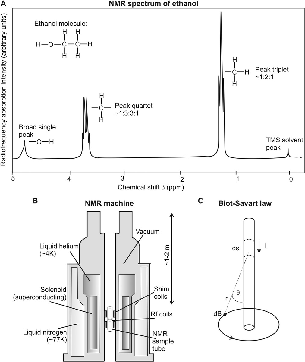
Figure 5.4 NMR spectroscopy. (a) Schematic of an NMR spectrum taken on with a “400 MHz” NMR machine in TMS solvent. (b) Schematic of a typical research NMR machine with double-skin Dewar. (c) Biot–Savart law: the contribution dB to the total circular B-field around an electrically conducting wire carrying current I can be calculated from the incremental element ds along the wire length of the length.
Thus, the single chemical shift peak for the C2 protons is split into a quartet of relative amplitude 1:3:3:1. The ratio of amplitudes in general is the (n + 1)th level of Pascal’s triangle (so a quintet multiplicity would have relative amplitudes of 1:4:6:4:1). Note also that J-coupling can also be detected through H-bonds, indicating some covalent character of hydrogen bonding at least. Observant readers might note from Figure 5.4a that there appears to be only a single peak corresponding to the 1H atom attached to the O atom of the –OH group, whereas from the simple logic earlier, one might expect a triplet O is covalently bonded to C2. However, the effects of J-coupling in this instance are largely lost and are similar for all 1H atoms in general, which are bound to heteroatoms (specifically, –OH and –NH groups) due to a rapid chemical transfer of a proton H+, allowing it to exchange with another proton from OH or NH in aqueous solution, which can occur even with tiny traces of water in a sample. This exchange process results in line broadening of all peaks in the hypothetical triplet, resulting in the appearance of a single broad peak.
5.4.4 Nuclear Relaxation
The transition from a high to low magnetic nuclear spin energy state in general is not a radiative process since the probability of spontaneous photon reemission varies as ν3, which is insignificant at radio frequencies. The two major processes, which affect the lifetime of an excited state, are spin–lattice relaxation and spin–spin relaxation, which are important in practical NMR spectroscopy since the absence of relaxation mechanisms would imply rapid saturation to high energy states and thus a small equivalent resonance absorption signal in a given sample.
Spin–spin relaxation (also known as “transverse relaxation”) involves coupling between nearby magnetic atomic nuclei, which have the same resonance frequency but which differ in their magnetic quantum numbers. It is also known as the “nuclear Overhauser effect” and, unlike J-coupling, is a free-space interaction not mediated through chemical bonds. A transition can occur in which the two magnetic quantum numbers are exchanged. There is therefore no change in the occupancy of energy states; however, this does decrease the “on” time probability of the excited state since an exchange in magnetic quantum number is equivalent to a transient misalignment of the magnetic dipole with the external B-field, which also broadens absorption peaks. Transient misalignment can also be caused by inhomogeneity in the B-field. The mean relaxation time associated with this process is denoted as T2. Solids can have T2 of a few milliseconds, while liquids more typically tens to hundreds of milliseconds.
Spin–lattice relaxation (also known as “longitudinal relaxation”) is due to a coupling between a spinning magnetic atomic nucleus and its surrounding lattice, for example, to collisions between mobile sample molecules and the solvent. This results in energy loss from the magnetic spin state and a consequent rise in temperature of the lattice. The mean relaxation time taken to return from an excited state back to the thermal equilibrium state is denoted T1. In general, T1 > T2, such that in normal nonviscous solvents at room temperature T1 ranges from ~0.1 to 20 s.
5.4.5 NMR in Practice
NMR often requires isotope enrichment, which can be technically rate limiting for investigations, in addition to typically tens of milligrams of purified sample, which can present a significant challenge in the case of many biomolecules, with liquid-state NMR requiring this to be dissolved in a few hundred microliters of pH-buffered solvent to produce high millimolar concentrations. To achieve the high B-fields required for NMR, with several machines capable of generating >20 T, magnets are based on a solenoid coil design. Early NMR magnets had an iron core and could generate fields strength up to ~5 T; however, most modern NMR machines, which can achieve maximum field strengths of ~6–24 T, utilize a superconducting solenoid, and some prototype machines using larger solenoids can operate in shorter pulses and generate higher transient B-fields, for example, up to ~100 T for millisecond-duration pulses.
Superconducting NMR solenoids of a coil length of ~100 km are composed of superconducting wire made usually from an alloy of niobium with tin and titanium, for example, (NbTaTi)3Sn, which is embedded in copper for mechanical stability and cooled to ~4 K using a liquid helium reservoir inside a Dewar, which is in turn thermally buffered from the room temperature environment by a second outer Dewar of liquid nitrogen (Figure 5.4b). The sample is lowered into the central solenoid bore, whose a diameter and length are both typically a few centimeters, which enclose transmitter/receiver radio frequency coils that surround the sample placed inside a narrow glass tube on the central solenoid axis. The size of the Dewars required result in such machines occupying the size of a room often requiring stair access to the sample’s entry port and the Dewar openings and are suitably expensive to purchase and maintain, necessitating an NMR facility infrastructure.
The B-field inside a long solenoid of length s, a coil current I, and a number of turns n can be modeled by the simple relation easily derived from the Biot–Savart law of (in reference to Figure 5.4c) dB = μ0I sin θds/(4 πr2):
(5.23)where μ0 is the vacuum permeability. The signal-to-noise ratio of an NMR measurement scales roughly as ~B3/2 (the bulk magnetization of the sample scales as ~B; see Worked Case Example 5.2, but the absorbed power also scales with ν, which scales with ~B, whereas the shot noise scales with ~√ν) so there is a motivation to generate higher fields. Field strengths of ~12 T are possible with solenoid cooling at 4 K, which corresponds to an ~500 MHz resonance frequency for 1H. To generate higher field strengths requires cooling lower than the ~4 K boiling point of helium, using the Joule–Thompson effect in a gas expansion unit to maintain solenoid temperatures as low as ~2 K, which can result in a coil current of a few hundred amperes, equivalent to a resonance frequency for 1H of up ~900 MHz.
Older NMR machines use a continuous wave (CW NMR) approach to sequentially probe the sample with different radio frequencies. The primary limitation with CW NMR is one of time, since multiple repeated spectra are usually required to improve signal-to-noise ratio, which can result in experiments taking several hours. Modern NMR machines use a frequency domain method known as “Fourier transform NMR (FT NMR),” which dramatically reduces the data acquisition time. Here, a sequence of short pulses of duration τ of a carrier wave of frequency f is composed of a range of frequency components, which span ~f ± 1/2πτ. The value of f used is catered to the unshielded resonance frequency of the magnetic atomic nucleus type under investigation, while τ is usually in the range 10−6 to 10−3 s to give sufficient frequency resolution to probe shifts in the resonance frequency of <0.1 ppm (typically ~0.02 ppm), with an averaged NMR spectroscopy trace typically taking less than 10 min to acquire.
As discussed previously, after the absorption of radio frequency energy, atomic nuclei relax back to a state of thermal equilibrium. This relaxation process involves the ultimate emission of tiny amounts of radio frequency energy from the high-energy-state nuclei. These tiny signals can be detected by radio frequency detector coils around the sample, and it is these that ultimately constitute the NMR signal.
5.4.6 NMR Spectroscopy Pulse Sequences
In practice, an NMR spectroscopy experiment is performed by using several repeated radiofrequency driving pulses, as opposed to continuous wave stimulation. However, different specific pulse sequences can generate different levels of information in regard to the spin relaxation processes. The simplest pulse sequence is just a single pulse followed by the detection of resonance signal, damped by relaxation (Figure 5.5a), known as the free induction decay (FID). The signal damping in this mode is exponential with a decay time referred to as
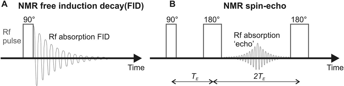
Figure 5.5 NMR spectroscopy pulse profiles. (a) Simple free induction decay. (b) Spin-echo pulse sequence (which is repeated multiple times on the same sample to allow averaging to improve the signal-to-noise ratio).
A pulse here is a superposition of oscillating radiofrequency waves (or spin packets) with a broad range of frequencies, which are used to rotate the bulk magnetization of the sample, which is set by the external B-field vector. Pulses are described as having a specific phase in terms of the angle of rotation of the bulk magnetization. So, for the simplest form of FID, a 90° pulse (referred to commonly as a “90” or “pi over two” pulse) is normally applied initially, with decay then resulting in dephasing 90° back to realignment of the bulk magnetization to its original orientation. This simple pulse sequence will normally be repeated to improve the signal-to-noise ratio. For analysis, this time-resolved repeating signal is usually Fourier transformed, resulting in a signal amplitude S, which depends on the relaxation time T1 as well as the time between pulse loops called the “repetition time” (TR):
(5.24)where k is a constant of proportionality with a density of spin nuclei in the sample given by ρ.
The spin-echo (SE) pulse sequence (also known as Hahn echo) is another common mode. Here, a sample is stimulated with two or more radio frequency pulses with subsequent detection of an echo resonance signal at some time after these initial pulses. Usually, this involves an initial 90° pulse, a wait period known as the echo time TE, then a 180° refocusing pulse, another wait period TE, then observation of the energy peak of the SE signal (Figure 5.5b)—the 180° pulse causes the magnetization to at least partially rephase, which results in the echo signal. On top of this are T1 and T2 relaxation processes, so the Fourier transformed signal is described by
(5.25)The enormous advantage of SE pulsing is that normally inhomogeneous relaxation processes will ultimately cause dephasing following repeating 90° pulsing, that is, different spin nuclei from the same atom types will start to precess at noticeably different rates, whereas the 180° pulse largely resets this dephasing back to zero, allowing more pulse loops before dephasing effects dominate, resulting in large effective increases in the signal-to-noise ratio.
The inversion recovery sequence is similar to SE pulsing, but here a 180° radio frequency pulse is initially applied. After a given time period known as the “inversion time” TI, during which time the bulk magnetization undergoes spin–lattice relaxation aligned 180° from the original vector, a 90o pulse is applied, which rotates the longitudinal magnetization into the XY plane. In this example, the 90° pulse is then applied, and the magnetization dephases giving an FID response as before. Normally, an inversion recovery sequence is then repeated every TR seconds to improve the signal-to-noise ratio, such that
(5.26)5.4.7 Multidimensional NMR
For complex biomolecules, often containing hundreds of atoms, overlapping peaks in a spectrum obtained using just a single magnetic atomic nucleus type, the so-called 1D-NMR, can make interpretation of the relative spatial localization of each different atom challenging. The correct assignment of atoms for structural determination of all the major classes of biomolecules is substantially improved by acquiring NMR spectra for one and then another type of magnetic atomic nuclei simultaneously, known as “multidimensional NMR” or “NMR correlation spectroscopy” (COSY). For example, the use of 2D-NMR with 13C and 15N isotopes can be used to generate a 2D heat map plot for chemical shift for each isotope plotted on each axis, with the 2D hotspots, as opposed to 1D peaks on their own, used to extract the molecular signature, which is particularly useful for identify backbone structures in proteins, a technique also referred to as “nuclear Overhauser effect spectroscopy” (NOESY). These correlative NMR approaches can be adapted in several multichannel NMR machines for 3D-NMR and 4D-NMR, with averaged spectra taking more like ~100 min to acquire.
Correlative NMR spectroscopy has been enormously successful in determining the structures of several types of biomolecules. These include complex lipids, carbohydrates, short nucleic acid sequences of ≲100 nucleotides, and peptides and proteins. The upper molecular weight limit for proteins using these NMR methods is ~35 kDa, which is comparatively small (e.g., an IgG antibody has a molecular weight of ~150 kDa). Multidimensional NMR can to a great extent overcome issues of overlapping chemical shift peaks associated with larger proteins; however, a larger issue is that the sample magnetization relaxes faster in large proteins, which ultimately sets a limit on the time to detect the NMR signal. Larger proteins have longer rotational correlation times and shorter transverse (T2) relaxation times, ultimately leading to line broadening in the NMR spectrum.
Transverse relaxation optimized spectroscopy (TROSY) has been used to overcome much of this line broadening. TROSY suppresses T2 relaxation in multidimensional NMR spectroscopy by using constructive interference between dipole–dipole coupling and anisotropic chemical shifts to produce much sharper chemical shift peaks. TROSY can also be used in combination with deuteration of larger proteins, that is, replacing 1H atoms with 2H, which further suppresses T2 relaxation. These improvements have allowed the structural determination of much larger proteins and protein complexes with nucleic acids, up to ~90 kDa.
NMR spectroscopy in its modern cutting-edge form has been used to great effect in obtaining atomic-level structures of several important biomolecules, especially of protein membranes. These are in general very difficult to crystallize, which is a requirement of the competing atomic-level structural determination technique of x-ray crystallography. A related spatially resolved technique used in biomedical in vivo diagnostics is magnetic resonance imaging (MRI), discussed in Chapter 7.
5.4.8 Electron Spin Resonance and Electron Paramagnetic Resonance
ESR, also referred to as EPR, relies on similar principles to NMR. However, here the resonance is from the absorption and emission of electromagnetic radiation due to transitions in the spin states of the electrons as opposed to magnetic atomic nuclei. This only occurs for an unpaired electron since paired electrons have a net spin of zero. ESR resonance peaks occur in the microwave range of ~10 GHz, with ESR spectrometers normally generating B-fields of ~1 T or less.
Unpaired electrons are chemically unstable, associated with highly reactive species such as free radicals. Such chemical species are short-lived, which limits the application of ESR, though this can be used to an advantage in that standard solvents do not give rise to a measurable ESR signal; therefore, the relative strength of the signal from the actual sample above this background solvent noise can be very high.
Site-directed spin labeling is a genetics technique that enables unpaired electron atom labels (i.e., spin labels) to be introduced into a protein. This uses a genetics technique called site-directed mutagenesis (discussed in more detail in Chapter 7). Here, specific labeling sites in the DNA genetic code of that protein are introduced. Once incorporated into the protein, a spin label’s motions are dictated by its local physical and chemical environment and give a very sensitive metric of molecular in the vicinity of the label. A common spin label is nitroxide, also known as “amine oxide” or “N-oxide,” which has a general chemical formula of R3N+–O− where R is a substituent organic chemical group, which contains an unpaired electron predominantly localized to the N–O bond, which has been used widely in the study of the structure and dynamics of large biomolecules using ESR.
5.4.9 Terahertz Radiation Applications and Spectroscopies
Terahertz radiation (T-rays) occupies a region of the electromagnetic spectrum between microwaves and infrared radiation, often referred to as the terahertz gap, where technologies for its generation and measurement are still in development. The fastest existing digital photon detectors have a bandwidth of a few tens of GHz, so the ~1011–1013 Hz characteristic frequencies of terahertz radiation (corresponding to wavelengths of ~30–3000 μm) are too high to be measured digitally but instead must be inferred indirectly, for example, by energy absorption measurements sampled at lower frequencies. However, the energy involved in transitions between different states in several fundamental biological processes has a characteristic equivalent resonance frequency in this terahertz range.
These include, for example, the collective vibrational motions of hydrogen-bonded nucleotide base pairs along the backbone of a DNA molecule, as well as many different molecular conformational changes in proteins, especially with a very high sensitivity to water, which is a useful metric for exposure of different molecular surfaces in a protein undergoing conformational changes. Terahertz spectroscopy, only developed at around the turn of the twentieth century, has yet to emerge into mainstream use in addressing practical biological questions (though for a good review of emerging applications, see Weightman, 2012). However, it has significant future potential for investigating a variety of biological systems.
Terahertz spectroscopy typically utilizes a rapid pulsed Ti–sapphire laser for generation of both terahertz radiation and detection. The laser output is in the near infrared; however, the pulse widths of these NIR wave packets are ~10−13 to 10−14 s, implying a frequency range of several terahertz, though centered on an NIR wavelength output of ~800 nm (~375 THz), which thus needs to be downshifted by two orders of magnitude.
A terahertz spectrometer is very similar in design to an FTIR spectrometer, in measuring the laser transmission in a cryofixed sample over a typical frequency range of ~0.3–10 THz. Samples are mounted in polyethylene holders, which are transparent to THz radiation, and held on an ultracooled stage at a temperature of ~4 K or less by liquid helium to minimize vibrational noise in the sample. THz spectroscopy has been applied in particular to investigating different topologies and flexibility of both DNA and RNA molecules in a cryofixed but physiologically relevant hydrated state, with an ability to detect base pair mutations in short oligonucleotide sequences from differences to the THz transmission spectra. THz spectroscopy can also be adapted to slow confocal scanning techniques across a thin sample, thus allowing terahertz imaging.
T-rays also have biophysical applications for tissue imaging. Intense T-rays can be controllably generated from a variety of sources, for example, both a synchrotron and free-electron laser (FEL) in addition to generating a continuum of x-ray radiation can be utilized to provide a stable source of T-rays, but also smaller sources that do require a very large facility such as lower power FEL sources or free-electron masers (which generate T-rays through cyclotron resonance of electrons in a device called a “gyrotron”), in this case due to high-frequency T-rays overlapping with low-frequency microwaves in the electromagnetic spectrum. Unlike x-rays, T-rays are nonionizing due to a lower photon energy and so do not result in the often high level of cellular damage of x-rays, especially due to damage of cellular DNA.
However, T-rays can penetrate into millimeters of biological tissues, which have low water content, such as fat, but have a high reflectivity for high water content tissues. Thus, T-rays can be used to measure tissue differences in water content, which has been used for the detection of various forms of epithelial cancer. Similarly, T-rays have been applied to generating more accurate images of teeth compared to x-rays in dentistry (see Chapter 7).
A recent application of T-rays has involved investigations of the structural states of the protein lysozyme, which was used as a model enzyme system (Lundholm et al., 2015). Here, the time-resolved structure of lysozyme was monitored at as low as ~1 K temperatures using x-ray crystallography, before and after bombarding the crystals with T-rays. Instead of being dissipated rapidly in a few nanoseconds as heat in the anticipated process of thermalization, the T-rays were absorbed in a spatially extended state of several coupled lysozyme molecules, extending the absorption lifetime to time scales three to six orders of magnitude longer than expected for single molecules. This coupled system is consistent with a state of condensed matter theoretically predicted in 1968 by Herbert Fröhlich (1968) as a possible theoretical mechanism for ordered energy storage in dielectric biomolecules in cell membranes, but never experimentally confirmed until now, called the Fröhlich condensate, which is the lowest order vibrational mode of condensed dielectric matter analogous to the Bose–Einstein condensate of a gas of bosons in quantum mechanics—in essence, long-range electrostatic Coulomb forces are coupled between molecules in a pool, resulting in coherent electrical oscillations, thus trapping absorbed energy of the right frequency (T-rays, in this case) for much longer than would be expected from individual electric dipole oscillations. The result is still being hotly debated as it could have enormous relevance to the existence of nontrivial quantum mechanical effects in many biological processes (see Chapter 9) and certainly may have implications for the real mode of operation of enzymes on their substrates, that is, potentially involving more physical-based processes cooperatively than what were imagined previously.
5.5 Tools that Use Gamma Rays, Radioisotope Decays, and Neutrons
Several other high-energy particles can be used as biophysical probes. Alpha and beta particles and gamma rays are relevant to the radioactive decay of isotopes, which can be used as reporter tags in biomolecules, especially useful in investigating the kinetics of biochemical processes. Gamma rays are also relevant to Mössbauer spectroscopy. Also, structural details of biomolecules can be investigated using the scattering/diffraction of thermal neutrons.
5.5.1 Mössbauer Spectroscopy
The Mössbauer effect consists of recoilless emission and absorption of gamma rays by/from an atomic nucleus in a solid or crystal lattice. When an excited nucleus emits a gamma ray, it must recoil to conserve momentum since the gamma ray photon has momentum. This implies that the emitted gamma ray photon has an energy, which is slightly too small to excite an equivalent atomic nucleus transition due to absorption of another identical atomic nucleus in the vicinity. However, if the gamma ray–emitting atomic nuclei are located inside a solid lattice, then, under sufficiently low temperatures, the atomic nucleus emitting the gamma ray photon cannot recoil individually but instead the effective recoil is that of the whole large lattice mass.
Under these conditions, the energy of a gamma ray photon may not be high enough to excite phonon energy loss through the whole lattice and therefore these results in negligible recoil energy loss of the emitted gamma ray photon. Thus, this photon can be absorbed by another identical atomic nucleus to excite an atomic nuclear transition, with consequent emission of a gamma ray photon, which therefore results in absorption resonance within the sample. However, in a similar way to the fine structure of NMR resonance peaks discussed previously in this chapter, the local chemical and physical environment can result in hyperfine splitting of the atomic nucleus energy transition levels in atomic nuclear energy levels (due to magnetic Zeeman splitting, quadrupole interactions, or isomer shifts, which are relevant to nonidentical atomic radii between absorber and emitter), but which can shift the resonance frequency by a much smaller amount than that observed in NMR, here by typically just one part in ~1012.
An important consequence of these small energy shifts, however, is that any relative motion between the source and absorber of speed around a few millimeters per second can result in comparable small shifts in the energy of the absorption lines; this can therefore result in absorption resonance in a manner that depends on the relative velocity between the gamma ray emission source and absorber. A typical Mössbauer spectrometer has a gamma ray source mounted on a drive, which can move at different velocities up to several millimeters per second, relative to a fixed absorber. A radiation Geiger counter is placed behind the absorber. When the source moves and Doppler shifting of the radiated energy occurs, resonance absorption in the fixed absorber decreases the measure transmission on the Geiger counter since excited nuclei reradiate over a time scale of ~10−7 s but isotropically.
Several candidate atomic isotopes are suitable for Mössbauer spectroscopy; however, the iron isotope 57Fe is ideal in having both a relatively low-energy gamma ray, which is a prerequisite for the Mössbauer effect, and relatively long-lived excited state, thus manifesting as a high-resonance signal-to-noise ratio. The cobalt isotope 57Co decays radioactively to 57Fe with emission of a 14.4 keV gamma ray photon and is thus typically used as the moving gamma ray source for performing 57Fe Mössbauer spectroscopy in the fixed absorber sample.
Iron is the most abundant transition metal in biological molecules and 57Fe Mössbauer spectroscopy has several biophysical applications, for example, biomolecules such as the oxygen carrier hemoglobin inside red blood cells, various essential enzymes in bacteria and plants, and also multicellular tissues that have high iron content, such as the liver and spleen. In essence, the information obtained from such experiments are very sensitive estimates for the number of distinct iron atom sites in the sample, along with their oxidation and spin states. Importantly, a Mössbauer spectrum is still observed regardless of the actual oxidation or spin state of the iron atoms, which differentiates from the EPR technique. These output parameters then allow predictions of molecular structure and function in the vicinity of the detected iron atoms to be made.
5.5.2 Radioisotope Decay
An example of a radioactive isotope (or radioisotope) in 57Co was discussed earlier in the context of being a gamma ray emitter in decaying to the more stable 57Fe isotope. But there are a range of different radioisotopes that have direct biophysical application in acting as a source of detectable radioactivity, which can be tagged onto a specific region of a biomolecule. This radioactive tag therefore acts as a biochemical reporter or tracer probe.
The kinetics of radioactivity can be modeled as a simple first-order process:
(5.27)where N is the number of radioisotopes of a specific type, with a decay constant λ. This results in a simple exponential decay for N. The half-life t1/2 is the time taken to reduce N by 50%, which is simple to demonstrate as ln 2/λ, while the mean lifetime of a given radioisotope is given by 1/λ.
The radioisotope is introduced in place of a normal relatively nonradioactive isotope, typically to detect components or metabolites in a biological system in time-resolved investigations. Radioisotopes have relatively unstable atomic nuclei and their presence can be detected from their emission of different specific types of radiation generated during the radioactive decay process in which an energetic lower energy (i.e., more stable) atomic nucleus is formed. The type of radiation produced depends on the isotope but can typically be detected by a Geiger counter or scintillation phosphor screen, often in combination with a CCD or PMT detector. In combination with stopped-flow techniques, biochemical reactions can be quenched at intermediate stages and the presence of radioisotopes measured in the detected metabolites, which thus allows a picture of the extent of different biochemical processes to be built up.
Common types of radiation emitted in radioisotope decay are gamma rays, beta particles (high-energy electrons), and alpha particles (4He2+, in other words helium nuclei with no atomic electrons). Alpha particles have a small depth of penetration (e.g., they are stopped by just a few centimeters of air) and are thus not useful as tracers but find application in radiotherapy. Common radioisotope tracers used in the life sciences include: 3H, 14C, 32P and 33P, 35S, 45Ca, and 125I. But 99mTc has a more focused application as a biomedical tracer. In addition, a number of radioisotopes decay with output of a positron, which are relevant as biomedical tracers in positron emission tomography, or PET (biomedical applications are discussed more generally in Chapter 7).
5.5.3 Neutron Diffraction and Small-Angle Scattering
Neutron diffraction works on similar principles to that of x-ray diffraction but utilizing an incident beam composed of thermal neutrons. Thermal neutrons can be generated by two principal methods. One is to use a thermal nuclear reactor. These utilize the fission of the 235U isotope, which releases an average of ~2.4 extra neutrons for every fission event. An example of 235U fission following neutron absorption is
(5.28)where just one of these released neutrons is required to sustain a chain reaction. Neutrons formed from uranium fission have an average energy of ~2 MeV. These neutrons are slowed down by a neutron moderator around the fission core (typically composed of water or graphite) so that emergent neutrons are in thermal equilibrium with their surroundings (hence, the term thermal neutrons), which have a mean energy of just ~0.025 eV with an equivalent de Broglie wavelength of ~0.2 nm.
The other approach to generating thermal neutrons is to use spallation neutron sources. These utilize particle accelerators and/or synchrotrons to generate intense, high-energy proton beams, which are directed at a heavy metal target (e.g., made from tantalum) whose impact can split the atomic nuclei to generate more neutrons. Proton synchrotron radiation impacted on such a metal target can generate >10 neutrons from a nuclear reactor, with an effective wavelength of ~10−10 m. Here, the scattering is due to interaction between the atomic nuclei as opposed to the electron cloud.
Neutron diffraction has a significant advantage over x-ray diffraction in that hydrogen atomic nuclei (i.e., single protons) will measurably scatter a neutron beam, and this scatter signal can be further enhanced by chemically replacing any solvent-accessible labile hydrogen atoms with deuterium, D, typically by solvating the target molecule in heavy water (D2O) rather than normal water (H2O) prior to crystallization. This allows the position of the hydrogen atoms to be measured directly, resulting in more accurate bond length predictions, but with disadvantages of requiring larger crystals (length ~1 mm) and a nearby nuclear reactor.
Small-angle neutron scattering (SANS) uses elastic scattering of thermal neutrons by a sample to generate structural information over a length scale of ~1–100 nm. The principles of operation are similar to SAXS performed with an incident x-ray beam. However, since neutrons scatter from atomic nuclei, unlike x-rays, which are scattered from atomic electron orbitals, the signal-to-noise ratio of diffraction intensity peaks is greater than SAXS for lower-atomic-number elements. SANS has been applied to determine the structural details of several macromolecular complexes, for example, including ribosomes and various biopolymer architectures such as the dendritic fibers of nerves in solution.
5.6 Summary Points
- EM is a powerful structural biology tool, but care must be taken to avoid overinterpretation from sample preparation artifacts.
- High-energy electrons, x-rays, and neutrons can be used in diffraction experiments to reveal atomic locations in biomolecules.
- X-ray crystallography is particularly useful for determining structures of biomolecules where large crystals with few imperfections can be grown, including many proteins and nucleic acid complexes.
- NMR spectroscopy results in a unique molecular signature and is particularly useful in determining structures of membrane-integrated proteins, which are difficult to crystallize.
- Diffraction techniques may also be extended to longer length scale investigations than single atoms, such as biological fibers.
Questions
- 5.1 A sample of a protein was prepared for TEM on a 120 keV machine using evaporative platinum rotary shadowing. A platinum atom is ~0.5 nm in diameter; however, the smallest observable metal particles were composed of five atoms.
- What is the practical spatial resolution in this experiment? The protein was known to exist in two structural states, A for 25% of the time and B for the rest of 75%. Each single TEM image of a protein was assigned as being in one of the two states so as to generate an average image from each subclass. Sequence data suggested the A–B transition results in a component of the molecule displacing by 5 nm.
- If each TEM images contains a mean of ~12 protein molecules, estimate how many images one would need to analyze to be able to measure this 5 nm translation change to at least a 5% accuracy.
- 5.2 A dehydrated cell membrane was placed in a 200 kV electron microscope normal to the beam of electrons, resulting in some of the transmitted electrons being diffracted as they passed through the membrane. A first-order diffraction peak was measured at a deflection angle of 3.5°. Estimate the lipid molecule separation in the cell membrane, stating any assumptions you make.
- 5.3 Over what range of accelerating voltage do classical and relativistic predictions for the matter wavelength of an electron agree to better than 1%?
- 5.4 What is an x-ray free-electron laser? Discuss the advantages that this tool has for determining structures of biological molecules over more traditional x-ray methods.
- 5.5 A single cell contains 1H atomic nuclei, which are mainly associated with water molecules, but with a significant number associated the –CH2– chemical motif found in lipids. A population of cells was homogenized and probed using 1H NMR spectroscopy in a “400 MHz” machine, which results in a 1.4 kHz difference in the resonance frequency between H2O and –CH2– protons. Estimate the equivalent chemical shift in units of ppm.
- 5.6 Why is NMR spectroscopy often described as the biophysical tool of choice for determining structures of membrane-integrated proteins?
- 5.7 A bespoke solenoid for an NMR spectroscopy device was constructed with a mean diameter of 50 mm by tightly winding an electrical wire of diameter 0.1 mm with a total length of 10 m. If a coil current of 5 A is run through the solenoid wire, estimate the average chemical shift of 1H atom in ethanol dissolved in TMS.
- 5.8 With reference to drawing a representative NMR spectrum, explain why the protons in an ethanol molecule are often categorized as being in one of three types, in terms of their response to nuclear magnetic resonance.
- 5.9 What is the “phase problem” in x-ray crystallography? How can it be overcome?
- 5.10 If the probability of a radioisotope decaying in small time Δt is equal to the number N1 of radioisotopes present multiplied by some constant λ1, develop an expression for the number of radioisotopes present after a general time t.
- What do we normally call λ1 for a general radioisotope?
- Derive a relation for the half-life and mean lifetime for these radioisotopes.
- This radioisotope was found to decay into a second radioisotope, of number in the sample denoted by N2, that decayed with a constant λ2 into a nonradioactive atom, of number N3 in the sample. Derive an expression for N3 as a function of time.
- Another radioactive decay chain was found to consist of several more (n − 2) radioactive intermediates from an initial radioisotope, before decaying to an nth that was not radioactive, with Nn atoms in the sample. Derive a general expression for Nn as a function of time, and comment on the relevance of one isotope in the chain having a significantly longer mean lifetime than the other in the series.
- 5.11 Electrons can be accelerated to far higher speeds than are currently used in modern electron microscopes, which therefore would have a smaller Bragg wavelength and better spatial resolution. Why then not use these to look at biological samples?
References
Key Reference
- Thibault, P. et al. (2008). High-resolution scanning x-ray diffraction microscopy. Science 321:379–382.
More Niche References
- Fröhlich, H. (1968). Long-range coherence and energy storage in biological systems. Int. J. Quant. Chem. 2:641–649.
- Gabor, D. (1948). A new microscopic principle. Nature 161:777–778.
- Humphry, M.J. et al. (2012). Ptychographic electron microscopy using high-angle dark-field scattering for sub-nanometre resolution imaging. Nat. Commun. 3:730.
- Leake, M.C. (2001). Investigation of the extensile properties of the giant sarcomeric protein titin by single-molecule manipulation using a laser-tweezers technique. PhD dissertation, London University, London.
- Lundholm, I.V. et al. (2015). Terahertz radiation induces non-thermal structural changes associated with Fröhlich condensation in a protein crystal. Struct. Dyn. 2:054702.
- Ortega, R. et al. (2012). X-ray absorption spectroscopy of biological samples. A tutorial. J. Anal. At. Spectrom. 27:2054–2065.
- Schneider, T.R. (2008). Synchrotron radiation: Micrometer-sized x-ray beams as fine tools for macromolecular crystallography. HFSP J. 2:302–306.
- Weightman, P. (2012). Prospects for the study of biological systems with high power sources of terahertz radiation. Phys. Biol. 9:053001.